Spline regression
Patsy offers a set of specific stateful transforms (for more details about stateful transforms see Stateful transforms) that you can use in formulas to generate splines bases and express non-linear fits.
General B-splines
B-spline bases can be generated with the bs() stateful
transform. The spline bases returned by bs() are designed to be
compatible with those produced by the R bs function.
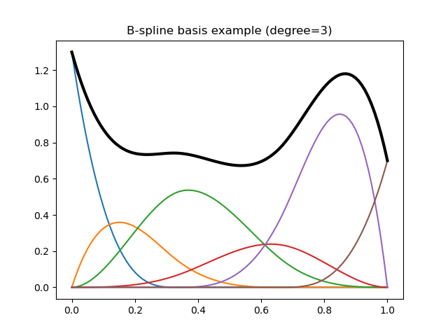
The following code illustrates a typical basis and the resulting spline:
In [1]: import matplotlib.pyplot as plt

In [2]: plt.title("B-spline basis example (degree=3)");

In [3]: x = np.linspace(0., 1., 100)

In [4]: y = dmatrix("bs(x, df=6, degree=3, include_intercept=True) - 1", {"x": x})

# Define some coefficients
In [5]: b = np.array([1.3, 0.6, 0.9, 0.4, 1.6, 0.7])

# Plot B-spline basis functions (colored curves) each multiplied by its coeff
In [6]: plt.plot(x, y*b);

# Plot the spline itself (sum of the basis functions, thick black curve)
In [7]: plt.plot(x, np.dot(y, b), color='k', linewidth=3);

In the following example we first set up our B-spline basis using some data and then make predictions on a new set of data:
In [8]: data = {"x": np.linspace(0., 1., 100)}

In [9]: design_matrix = dmatrix("bs(x, df=4)", data)

In [10]: new_data = {"x": [0.1, 0.25, 0.9]}

In [11]: build_design_matrices([design_matrix.design_info], new_data)[0]
Out[11]:
DesignMatrix with shape (3, 5)
  Intercept  bs(x, df=4)[0]  bs(x, df=4)[1]  bs(x, df=4)[2]  bs(x, df=4)[3]
          1         0.43400           0.052         0.00200           0.000
          1         0.59375           0.250         0.03125           0.000
          1         0.00200           0.052         0.43400           0.512
  Terms:
    'Intercept' (column 0)
    'bs(x, df=4)' (columns 1:5)
bs() can produce B-spline bases of arbitrary degrees – e.g.,
degree=0 will give produce piecewise-constant functions,
degree=1 will produce piecewise-linear functions, and the default
degree=3 produces cubic splines. The next section describes more
specialized functions for producing different types of cubic splines.
Natural and cyclic cubic regression splines
Natural and cyclic cubic regression splines are provided through the stateful
transforms cr() and cc() respectively. Here the spline is
parameterized directly using its values at the knots. These splines were designed
to be compatible with those found in the R package
mgcv
(these are called cr, cs and cc in the context of mgcv), but
can be used with any model.
Warning
Note that the compatibility with mgcv applies only to the generation of spline bases: we do not implement any kind of mgcv-compatible penalized fitting process. Thus these spline bases can be used to precisely reproduce predictions from a model previously fitted with mgcv, or to serve as building blocks for other regression models (like OLS).
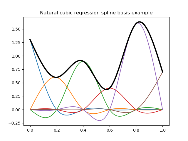
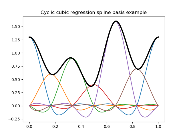
Here are some illustrations of typical natural and cyclic spline bases:
In [12]: plt.title("Natural cubic regression spline basis example");

In [13]: y = dmatrix("cr(x, df=6) - 1", {"x": x})

# Plot natural cubic regression spline basis functions (colored curves) each multiplied by its coeff
In [14]: plt.plot(x, y*b);

# Plot the spline itself (sum of the basis functions, thick black curve)
In [15]: plt.plot(x, np.dot(y, b), color='k', linewidth=3);

In [16]: plt.title("Cyclic cubic regression spline basis example");

In [17]: y = dmatrix("cc(x, df=6) - 1", {"x": x})

# Plot cyclic cubic regression spline basis functions (colored curves) each multiplied by its coeff
In [18]: plt.plot(x, y*b);

# Plot the spline itself (sum of the basis functions, thick black curve)
In [19]: plt.plot(x, np.dot(y, b), color='k', linewidth=3);

In the following example we first set up our spline basis using same data as for the B-spline example above and then make predictions on a new set of data:
In [20]: design_matrix = dmatrix("cr(x, df=4, constraints='center')", data)

In [21]: new_design_matrix = build_design_matrices([design_matrix.design_info], new_data)[0]

In [22]: new_design_matrix
Out[22]:
DesignMatrix with shape (3, 5)
  Columns:
    ['Intercept',
     "cr(x, df=4, constraints='center')[0]",
     "cr(x, df=4, constraints='center')[1]",
     "cr(x, df=4, constraints='center')[2]",
     "cr(x, df=4, constraints='center')[3]"]
  Terms:
    'Intercept' (column 0)
    "cr(x, df=4, constraints='center')" (columns 1:5)
  (to view full data, use np.asarray(this_obj))

In [23]: np.asarray(new_design_matrix)
Out[23]:
array([[ 1.        ,  0.15855682, -0.5060419 , -0.40944318, -0.16709613],
       [ 1.        ,  0.71754625, -0.22956933, -0.28245375, -0.10215042],
       [ 1.        , -0.1602992 , -0.30354568,  0.4077008 ,  0.43900769]])
Note that in the above example 5 knots are actually used to achieve 4 degrees of freedom since a centering constraint is requested.
Note that the API is different from mgcv:
In patsy one can specify the number of degrees of freedom directly (actual number of columns of the resulting design matrix) whereas in mgcv one has to specify the number of knots to use. For instance, in the case of cyclic regression splines (with no additional constraints) the actual degrees of freedom is the number of knots minus one.
In patsy one can specify inner knots as well as lower and upper exterior knots which can be useful for cyclic spline for instance.
In mgcv a centering/identifiability constraint is automatically computed and absorbed in the resulting design matrix. The purpose of this is to ensure that if
bis the array of initial parameters (corresponding to the initial unconstrained design matrixdm), our model is centered, ienp.mean(np.dot(dm, b))is zero. We can rewrite this asnp.dot(c, b)being zero withca 1-row constraint matrix containing the mean of each column ofdm. Absorbing this constraint in the final design matrix means that we rewrite the model in terms of unconstrained parameters (this is done through a QR-decomposition of the constraint matrix). Those unconstrained parameters have the property that when projected back into the initial parameters space (let’s callb_backthe result of this projection), the constraintnp.dot(c, b_back)being zero is automatically verified. In patsy one can choose between no constraint, a centering constraint like mgcv ('center') or a user provided constraint matrix.
Tensor product smooths
Smooths of several covariates can be generated through a tensor product of
the bases of marginal univariate smooths. For these marginal smooths one can
use the above defined splines as well as user defined smooths provided they
actually transform input univariate data into some kind of smooth functions
basis producing a 2-d array output with the (i, j) element corresponding
to the value of the j th basis function at the i th data point.
The tensor product stateful transform is called te().
Note
The implementation of this tensor product is compatible with mgcv when considering only cubic regression spline marginal smooths, which means that generated bases will match those produced by mgcv. Recall that we do not implement any kind of mgcv-compatible penalized fitting process.
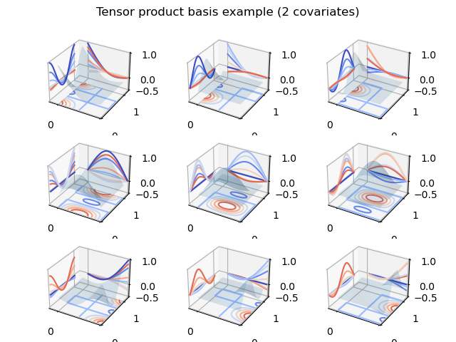
In the following code we show an example of tensor product basis functions
used to represent a smooth of two variables x1 and x2. Note how
marginal spline bases patterns can be observed on the x and y contour projections:
In [24]: from matplotlib import cm

In [25]: from mpl_toolkits.mplot3d.axes3d import Axes3D

In [26]: x1 = np.linspace(0., 1., 100)

In [27]: x2 = np.linspace(0., 1., 100)

In [28]: x1, x2 = np.meshgrid(x1, x2)

In [29]: df = 3

In [30]: y = dmatrix("te(cr(x1, df), cc(x2, df)) - 1",
   ....:            {"x1": x1.ravel(), "x2": x2.ravel(), "df": df})
   ....:

In [31]: print(y.shape)
(10000, 9)

In [32]: fig = plt.figure()

In [33]: fig.suptitle("Tensor product basis example (2 covariates)");

In [34]: for i in range(df * df):
   ....:     ax = fig.add_subplot(df, df, i + 1, projection='3d')
   ....:     yi = y[:, i].reshape(x1.shape)
   ....:     ax.plot_surface(x1, x2, yi, rstride=4, cstride=4, alpha=0.15)
   ....:     ax.contour(x1, x2, yi, zdir='z', cmap=cm.coolwarm, offset=-0.5)
   ....:     ax.contour(x1, x2, yi, zdir='y', cmap=cm.coolwarm, offset=1.2)
   ....:     ax.contour(x1, x2, yi, zdir='x', cmap=cm.coolwarm, offset=-0.2)
   ....:     ax.set_xlim3d(-0.2, 1.0)
   ....:     ax.set_ylim3d(0, 1.2)
   ....:     ax.set_zlim3d(-0.5, 1)
   ....:     ax.set_xticks([0, 1])
   ....:     ax.set_yticks([0, 1])
   ....:     ax.set_zticks([-0.5, 0, 1])
   ....:

In [35]: fig.tight_layout()

Following what we did for univariate splines in the preceding sections, we will now set up a 3-d smooth basis using some data and then make predictions on a new set of data:
In [36]: data = {"x1": np.linspace(0., 1., 100),
   ....:         "x2": np.linspace(0., 1., 100),
   ....:         "x3": np.linspace(0., 1., 100)}
   ....:

In [37]: design_matrix = dmatrix("te(cr(x1, df=3), cr(x2, df=3), cc(x3, df=3), constraints='center')",
   ....:                         data)
   ....:

In [38]: new_data = {"x1": [0.1, 0.2],
   ....:             "x2": [0.2, 0.3],
   ....:             "x3": [0.3, 0.4]}
   ....:

In [39]: new_design_matrix = build_design_matrices([design_matrix.design_info], new_data)[0]

In [40]: new_design_matrix
Out[40]:
DesignMatrix with shape (2, 27)
  Columns:
    ['Intercept',
     "te(cr(x1, df=3), cr(x2, df=3), cc(x3, df=3), constraints='center')[0]",
     "te(cr(x1, df=3), cr(x2, df=3), cc(x3, df=3), constraints='center')[1]",
     "te(cr(x1, df=3), cr(x2, df=3), cc(x3, df=3), constraints='center')[2]",
     "te(cr(x1, df=3), cr(x2, df=3), cc(x3, df=3), constraints='center')[3]",
     "te(cr(x1, df=3), cr(x2, df=3), cc(x3, df=3), constraints='center')[4]",
     "te(cr(x1, df=3), cr(x2, df=3), cc(x3, df=3), constraints='center')[5]",
     "te(cr(x1, df=3), cr(x2, df=3), cc(x3, df=3), constraints='center')[6]",
     "te(cr(x1, df=3), cr(x2, df=3), cc(x3, df=3), constraints='center')[7]",
     "te(cr(x1, df=3), cr(x2, df=3), cc(x3, df=3), constraints='center')[8]",
     "te(cr(x1, df=3), cr(x2, df=3), cc(x3, df=3), constraints='center')[9]",
     "te(cr(x1, df=3), cr(x2, df=3), cc(x3, df=3), constraints='center')[10]",
     "te(cr(x1, df=3), cr(x2, df=3), cc(x3, df=3), constraints='center')[11]",
     "te(cr(x1, df=3), cr(x2, df=3), cc(x3, df=3), constraints='center')[12]",
     "te(cr(x1, df=3), cr(x2, df=3), cc(x3, df=3), constraints='center')[13]",
     "te(cr(x1, df=3), cr(x2, df=3), cc(x3, df=3), constraints='center')[14]",
     "te(cr(x1, df=3), cr(x2, df=3), cc(x3, df=3), constraints='center')[15]",
     "te(cr(x1, df=3), cr(x2, df=3), cc(x3, df=3), constraints='center')[16]",
     "te(cr(x1, df=3), cr(x2, df=3), cc(x3, df=3), constraints='center')[17]",
     "te(cr(x1, df=3), cr(x2, df=3), cc(x3, df=3), constraints='center')[18]",
     "te(cr(x1, df=3), cr(x2, df=3), cc(x3, df=3), constraints='center')[19]",
     "te(cr(x1, df=3), cr(x2, df=3), cc(x3, df=3), constraints='center')[20]",
     "te(cr(x1, df=3), cr(x2, df=3), cc(x3, df=3), constraints='center')[21]",
     "te(cr(x1, df=3), cr(x2, df=3), cc(x3, df=3), constraints='center')[22]",
     "te(cr(x1, df=3), cr(x2, df=3), cc(x3, df=3), constraints='center')[23]",
     "te(cr(x1, df=3), cr(x2, df=3), cc(x3, df=3), constraints='center')[24]",
     "te(cr(x1, df=3), cr(x2, df=3), cc(x3, df=3), constraints='center')[25]"]
  Terms:
    'Intercept' (column 0)
    "te(cr(x1, df=3), cr(x2, df=3), cc(x3, df=3), constraints='center')" (columns 1:27)
  (to view full data, use np.asarray(this_obj))

In [41]: np.asarray(new_design_matrix)
Out[41]:
array([[ 1.00000000e+00,  3.50936277e-01, -2.42388845e-02,
         2.79787994e-02,  3.82596528e-01, -2.22904932e-02,
        -4.12367917e-04, -5.83969029e-02,  9.25602506e-03,
        -1.93080061e-03,  1.13410128e-01,  2.40550675e-03,
         1.44263739e-02,  3.13527293e-02, -1.48712359e-01,
        -2.12892006e-02, -8.23983725e-03, -3.41861279e-02,
         3.77323208e-03, -2.07265029e-02,  5.80002506e-03,
        -2.15508006e-02, -1.05942372e-02, -3.39701279e-02,
        -6.27553548e-02,  1.46393875e-02, -3.00859954e-02],
       [ 1.00000000e+00,  1.09386577e-01,  4.93985311e-02,
        -8.80045587e-02,  3.34907265e-01,  1.14474114e-01,
         1.58055508e-02, -4.16223930e-02, -7.14533704e-03,
        -5.02445587e-02,  1.15899265e-01,  5.97221139e-02,
        -7.67240826e-02,  2.54852719e-01, -5.82470575e-02,
        -1.38925587e-02, -3.09397741e-02, -5.69908474e-02,
         1.19655508e-02, -1.93503930e-02, -1.57733704e-03,
        -1.19725587e-02, -4.20757741e-02, -5.97748474e-02,
        -7.82200162e-02,  2.04894751e-02, -3.43123674e-02]])