Image Registration

The dtcwt.registration module provides an implementation of a DTCWT-based image registration algorithm. The output is similar, but not identical, to “optical flow”. The underlying assumption is that the source image is a smooth locally-affine warping of a reference image. This assumption is valid in some classes of medical image registration and for video sequences with small motion between frames.

Algorithm overview

This section provides a brief overview of the algorithm itself. The algorithm is a 2D version of the 3D registration algorithm presented in Efficient Registration of Nonrigid 3-D Bodies. The motion field between two images is a vector field whose elements represent the direction and distance of displacement for each pixel in the source image required to map it to a corresponding pixel in the reference image. In this algorithm the motion is described via the affine transform which can represent rotation, translation, shearing and scaling. An advantage of this model is that if the motion of two neighbouring pixels are from the same model then they will share affine transform parameters. This allows for large regions of the image to be considered as a whole and helps mitigate the aperture problem.

The model described below is based on the model in Phase-based multidimensional volume registration with changes designed to allow use of the DTCWT as a front end.

Motion constraint

The three-element homogeneous displacement vector at location \(\mathbf{x}\) is defined to be

\[\begin{split}\mathbf{\tilde{v}}(\mathbf{x}) \equiv \begin{bmatrix} \mathbf{v}(\mathbf{x}) \\ 1 \end{bmatrix}\end{split}\]

where \(\mathbf{v}(\mathbf{x})\) is the motion vector at location \(\mathbf{x} = [ x \, y ]^T\). A motion constraint is a three-element vector, \(\mathbf{c}(\mathbf{x})\) such that

\[\mathbf{c}^T(\mathbf{x}) \, \mathbf{\tilde{v}}(\mathbf{x}) = 0.\]

In the two-dimensional DTCWT, the phase of each complex highpass coefficient has an approximately linear relationship with the local shift vector. We can therefore write

\[\frac{\partial \theta_d}{\partial t} = \nabla_\mathbf{x} \theta_d \cdot \mathbf{v}(\mathbf{x})\]

where \(\nabla_\mathbf{x} \theta_d \equiv [(\partial \theta_d/\partial x) \, (\partial \theta_d/\partial y)]^T\) and represents the phase gradient at \(\mathbf{x}\) for subband \(d\) in both of the \(x\) and \(y\) directions.

Numerical estimation of the partial derivatives of \(\theta_d\) can be performed by noting that multiplication of a subband pixels’s complex coefficient by the conjugate of its neighbour subtracts phase whereas multiplication by the neighbour adds phase. We can thus construct equivalents of forward-, backward- and central difference algorithms for phase gradients.

Comparing the relations above, it is clear that the motion constraint vector, \(\mathbf{c}_d(\mathbf{x})\), corresponding to subband \(d\) at location \(\mathbf{x}\) satisfies the following:

\[\begin{split}\mathbf{c}_d(\mathbf{x}) = C_d(\mathbf{x}) \begin{bmatrix} \nabla_\mathbf{x} \theta_d \\ - \frac{\partial \theta_d}{\partial t} \end{bmatrix}\end{split}\]

where \(C_d(\mathbf{x})\) is some weighting factor which we can interpret as a measure of the confidence we have of subband \(d\) specifying the motion at \(\mathbf{x}\).

This confidence measure can be heuristically designed. The measure used in this implementation is:

\[C_d(\mathbf{x}) = \frac{ \left| \sum_{k=1}^4 u_k^* v_k \right|^2 }{ \sum_{k=1}^4 (\left|u_k\right|^3 + \left|v_k\right|^3) + \epsilon }.\]

where \(u_k\) and \(v_k\) are the wavelet coefficients in the reference and source transformed images, subscripts \(k = 1 \dots 4\) denote the four diagonally neighbouring coefficients and \(\epsilon\) is some small value to avoid division by zero when the wavelet coefficients are small. It is beyond the scope of this documentation to describe the design of this metric. Refer to the original paper for more details.

Cost function

The model is represented via the six parameters \(a_1 \dots a_6\) such that

\[\begin{split}\mathbf{v}(\mathbf{x}) = \begin{bmatrix} 1 & 0 & x & 0 & y & 0 \\ 0 & 1 & 0 & x & 0 & y \end{bmatrix} \begin{bmatrix} a_1 \\ \vdots \\ a_6 \end{bmatrix} \equiv \mathbf{K}(\mathbf{x}) \, \mathbf{a}.\end{split}\]

We then make the following definitions:

\[\begin{split}\mathbf{\tilde{K}}(\mathbf{x}) \equiv \begin{bmatrix} \mathbf{K}(\mathbf{x}) & \mathbf{0} \\ \mathbf{0} & 1 \end{bmatrix}, \quad \mathbf{\tilde{a}} \equiv \begin{bmatrix} \mathbf{a} \\ 1 \end{bmatrix}\end{split}\]

and then the homogenous motion vector is given by

\[\mathbf{\tilde{v}}(\mathbf{x}) = \mathbf{\tilde{K}}(\mathbf{x}) \, \mathbf{\tilde{a}}.\]

Considering all size subband directions, we have:

\[\mathbf{c}_d(\mathbf{x}) \, \mathbf{\tilde{K}}(\mathbf{x}) \, \mathbf{\tilde{a}} = 0, \quad \forall \ d \in \left\{ 1, \dots, 6 \right\}.\]

Each location \(\mathbf{x}\) has six constraint equations for six unknown affine parameters in \(\mathbf{\tilde{a}}\). We can solve for \(\mathbf{\tilde{a}}\) by minimising squared error \(\epsilon(\mathbf{x})\):

\[\begin{split}\begin{aligned} \epsilon(\mathbf{x}) &= \sum_{d=1}^6 \left\| \mathbf{c}_d^T(\mathbf{x}) \mathbf{\tilde{K}}(\mathbf{x}) \mathbf{\tilde{a}} \right\|^2 \\ &= \sum_{d=1}^6 \mathbf{\tilde{a}}^T \, \mathbf{\tilde{K}}^T(\mathbf{x}) \, \mathbf{c}_d(\mathbf{x}) \mathbf{c}^T_d(\mathbf{x}) \, \mathbf{\tilde{K}}(\mathbf{x}) \, \mathbf{\tilde{a}} \\ &= \mathbf{\tilde{a}}^T \mathbf{\tilde{Q}}(\mathbf{x}) \mathbf{\tilde{a}} \end{aligned}\end{split}\]

where

\[\mathbf{\tilde{Q}}(\mathbf{x}) \equiv \sum_{d=1}^6 \mathbf{\tilde{K}}^T(\mathbf{x}) \, \mathbf{c}_d(\mathbf{x}) \mathbf{c}^T_d(\mathbf{x}) \, \mathbf{\tilde{K}}(\mathbf{x}).\]

In practice, in order to handle the registration of dissimilar image features and also to handle the aperture problem, it is helpful to combine \(\mathbf{\tilde{Q}}(\mathbf{x})\) matrices across more than one level of DTCWT and over a slightly wider area within each level. This results in better estimates of the affine parameters and reduces the likelihood of obtaining singular matrices. We define locality \(\mathbf{\chi}\) to represent this wider spatial and inter-scale region, such that

\[\mathbf{\tilde{Q}}_\mathbf{\chi} = \sum_{\mathbf{x} \in \mathbf{\chi}} \mathbf{\tilde{Q}}(\mathbf{x}).\]

The \(\mathbf{\tilde{Q}}_\mathbf{\chi}\) matrices are symmetric and so can be written in the following form:

\[\begin{split}\mathbf{\tilde{Q}}_\mathbf{\chi} = \begin{bmatrix} \mathbf{Q}_\mathbf{\chi} & \mathbf{q}_\mathbf{\chi} \\ \mathbf{q}^T_\mathbf{\chi} & q_{0,\mathbf{\chi}} \end{bmatrix}\end{split}\]

where \(\mathbf{q}_\mathbf{\chi}\) is a six-element vector and \(q_{0,\mathbf{\chi}}\) is a scalar. Substituting into our squared error function gives

\[\epsilon_\mathbf{\chi} = \mathbf{a}^T \mathbf{Q}_\mathbf{\chi} \mathbf{a} + 2 \mathbf{a}^T \mathbf{q}_\mathbf{\chi} + q_{0,\mathbf{\chi}}.\]

To minimize, we differentiate and set to zero. Hence,

\[\nabla_\mathbf{a} \epsilon_\mathbf{\chi} = 2 \mathbf{Q}_\mathbf{\chi} \mathbf{a} + 2 \mathbf{q}_\mathbf{\chi} = 0\]

and so the local affine parameter vector satisfies

\[\mathbf{Q}_\mathbf{\chi} \mathbf{a}_\mathbf{\chi} = - \mathbf{q}_\mathbf{\chi}.\]

In our implementation, we avoid calculating the inverse of \(\mathbf{Q}_\mathbf{\chi}\) directly and solve this equation by eigenvector decomposition.

Iteration

There are three stres in the full registration algorithm: transform the images to the DTCWT domain, perform motion estimation and register the source image. We do this via an iterative process where coarse-scale estimates of \(\mathbf{a}_\mathbf{\chi}\) are estimated from coarse-scale levels of the transform and progressively refined with finer-scale levels.

The following flow diagram, taken from the paper, illustrates the algorithm.

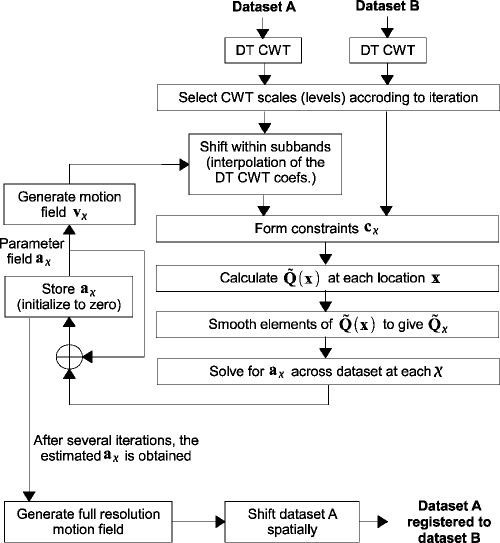
The pair of images to be registered are first transformed by the DTCWT and levels to be used for motion estimation are selected. The subband coefficients of the source image are shifted according to the current motion field estimate. These shifted coefficients together with those of the reference image are then used to generate motion constraints. From these the \(\mathbf{\tilde{Q}}_\mathbf{\chi}\) matrices are calculated and the local affine distortion parameters updated. After a few iterations, the distortion parameters are used to warp the source image directly.

Using the implementation

The implementation of the image registration algorithm is accessed via the dtcwt.registration module’s functions. The two functions of most interest at dtcwt.registration.estimatereg() and dtcwt.registration.warp(). The former will estimate \(\mathbf{a}_\mathbf{\chi}\) for each 8x8 block in the image and dtcwt.registration.warp() will take these affine parameter vectors and warp an image with them.

As an example, we will register two frames from a video of road traffic. Firstly, as boilerplate, import plotting command from pylab and also the datasets module which is part of the test suite for dtcwt.

from pylab import *
import datasets

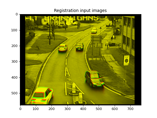
If we show one image in the red channel and one in the green, we can see where the images are incorrectly registered by looking for red or green fringes:

ref, src = datasets.regframes('traffic')

figure()
imshow(np.dstack((ref, src, np.zeros_like(ref))))
title('Registration input images')

(Source code, png, hires.png, pdf)

To register the images we first take the DTCWT:

import dtcwt

transform = dtcwt.Transform2d()
ref_t = transform.forward(ref, nlevels=6)
src_t = transform.forward(src, nlevels=6)

Registration is now performed via the dtcwt.registration.estimatereg() function. Once the registration is estimated, we can warp the source image to the reference using the dtcwt.registration.warp() function.

import dtcwt.registration as registration

reg = registration.estimatereg(src_t, ref_t)
warped_src = registration.warp(src, reg, method='bilinear')

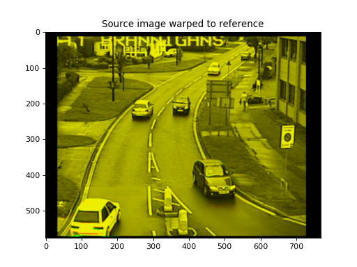
Plotting the warped and reference image in the green and red channels again shows a marked reduction in colour fringes.

figure()

imshow(np.dstack((ref, warped_src, np.zeros_like(ref))))
title('Source image warped to reference')

(Source code, png, hires.png, pdf)

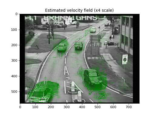
The velocity field, in units of image width/height, can be calculated by the dtcwt.registration.velocityfield() function. We need to scale the result by the image width and height to get a velocity field in pixels.

vxs, vys = registration.velocityfield(reg, ref.shape[:2], method='bilinear')
vxs = vxs * ref.shape[1]
vys = vys * ref.shape[0]

We can plot the result as a quiver map overlaid on the reference image:

figure()

X, Y = np.meshgrid(np.arange(ref.shape[1]), np.arange(ref.shape[0]))

imshow(ref, cmap=cm.gray, clim=(0,1))

step = 8

quiver(X[::step,::step], Y[::step,::step],
       vxs[::step,::step], vys[::step,::step],
       color='g', angles='xy', scale_units='xy', scale=0.25)

title('Estimated velocity field (x4 scale)')

(Source code, png, hires.png, pdf)

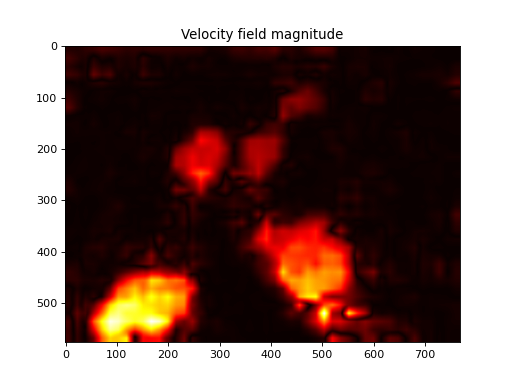
We can also plot the magnitude of the velocity field which clearly shows the moving cars:

figure()
imshow(np.abs(vxs + 1j*vys), cmap=cm.hot)
title('Velocity field magnitude')

(Source code, png, hires.png, pdf)