What’s New in Astropy 5.2?
Overview
Astropy 5.2 is a major release that adds significant new functionality since the 5.1 release.
In particular, this release includes:
In addition to these major changes, Astropy 5.2 includes a large number of smaller improvements and bug fixes, which are described in the Full change log. By the numbers:
1065 commits have been added since 5.1
157 issues have been closed since 5.1
320 pull requests have been merged since 5.1
50 people have contributed since 5.1
18 of which are new contributors
Quantity data types
The default dtype argument for Quantity has been changed, so that one can
now explicitly give dtype=None to get the same behaviour as numpy.
Without an explicit argument, any integer values are still upcast to floating
point, since that makes more sense for physical quantities.
Updates to astropy.cosmology
A new comparison function has been added –
astropy.cosmology.cosmology_equal() – that mirrors its numpy counterparts
but allows for the arguments to be converted to a Cosmology and to compare flat
cosmologies with their non-flat equivalents.
>>> from astropy.cosmology import cosmology_equal
>>> from astropy.cosmology import FlatLambdaCDM, LambdaCDM
>>> cosmo1 = FlatLambdaCDM(70, 0.3)
>>> cosmo2 = LambdaCDM(70, 0.3, 0.7)
>>> cosmology_equal(cosmo1.to_format("mapping"), cosmo2,
...                 format=("mapping", None), allow_equivalent=True)
True
A cosmology can be parsed from or converted to a HTML table using
the new HTML methods in Cosmology’s to/from_format I/O.
>>> from astropy.cosmology import Planck18
>>> Planck18.write("planck18.html")
The columns can be latex/mathjax formatted using the flag latex_names=True;
then if the following is added to the file’s header, the column names will
render nicely.:
<script
src="https://polyfill.io/v3/polyfill.min.js?features=es6"></script>
<script type="text/javascript" id="MathJax-script" async
    src="https://cdn.jsdelivr.net/npm/mathjax@3/es5/tex-chtml.js">
</script>
Topocentric ITRS Frame
A topocentric ITRS frame has been added that makes dealing with near-Earth objects easier and more intuitive.:
>>> from astropy.coordinates import EarthLocation, AltAz, ITRS
>>> from astropy.time import Time
>>> from astropy import units as u

>>> t = Time('J2010')
>>> obj = EarthLocation(-1*u.deg, 52*u.deg, height=10.*u.km)
>>> home = EarthLocation(-1*u.deg, 52*u.deg, height=0.*u.km)

>>> # Direction of object from GEOCENTER
>>> itrs_geo = obj.get_itrs(t).cartesian

>>> # now get the Geocentric ITRS position of observatory
>>> obsrepr = home.get_itrs(t).cartesian

>>> # topocentric ITRS position of a straight overhead object
>>> itrs_repr = itrs_geo - obsrepr

>>> # create an ITRS object that appears straight overhead for a TOPOCENTRIC OBSERVER
>>> itrs_topo = ITRS(itrs_repr, obstime=t, location=home)

>>> # convert to AltAz
>>> aa = itrs_topo.transform_to(AltAz(obstime=t, location=home))
Performance Improvements
To help speed up coordinate transformations, several performance improvements
were implemented, mainly concerning validity checks in Angle and
how FrameAttributes are accessed.
Performance improvements will vary between different tasks, e.g., the speedup of
transforming AltAz coordinates to
ICRS is 5-10 % depending on the number of coordinates.
Enhanced Fixed Width ASCII Tables
It is now possible to read and write a fixed width ASCII table that includes
additional header rows specifying any or all of the column dtype, unit,
format, and description. This is available in the fixed_width and
fixed_width_two_line formats via the new header_rows keyword argument:
>>> from astropy.io import ascii
>>> from astropy.table.table_helpers import simple_table
>>> dat = simple_table(size=3, cols=4)
>>> dat["b"].info.unit = "m"
>>> dat["d"].info.unit = "m/s"
>>> dat["b"].info.format = ".2f"
>>> ascii.write(
...     dat,
...     format="fixed_width_two_line",
...     header_rows=["name", "unit", "format"]
... )
a    b c     d
     m   m / s
   .2f
- ---- - -----
1 1.00 c     4
2 2.00 d     5
3 3.00 e     6
Accessing cloud-hosted FITS files
A use_fsspec argument has been added to astropy.io.fits.open which
enables users to seamlessly extract data from FITS files stored on a web server
or in the cloud without downloading the entire file to local storage.
This feature uses a new optional dependency, fsspec, which supports a range
of remote and distributed storage backends including Amazon and Google Cloud Storage.
For example, you can now access a Hubble Space Telescope image located in
Hubble’s public Amazon S3 bucket as follows:
>>> from astropy.io import fits
>>> uri = "s3://stpubdata/hst/public/j8pu/j8pu0y010/j8pu0y010_drc.fits"
>>> with fits.open(uri, fsspec_kwargs={"anon": True}) as hdul:
...
...     # Download a single header
...     header = hdul[1].header
...
...     # Download a single image
...     mydata = hdul[1].data
...
...     # Download a small cutout
...     cutout = hdul[1].section[10:20, 30:50]
Note that the example above obtains a cutout image using the section
attribute rather than the traditional data attribute.
The use of .section ensures that only the necessary parts of the FITS
image are transferred from the server, rather than downloading the entire data
array. This trick can significantly speed up your code if you require small
subsets of large FITS files located on slow (remote) storage systems.
See Obtaining subsets from cloud-hosted FITS files for additional information on working with
FITS files in this way.
Drawing the instrument beam and a physical scale bar on celestial images
Two functions have been added to wcsaxes: add_beam() and
add_scalebar(). These functions allow to draw the shape of the instrument beam (e.g.for radio
observations) and a physical scale bar on celestial images:
>>> from astropy.io import fits
>>> from astropy.wcs import WCS
>>> from astropy import units as u
>>> from astropy.visualization.wcsaxes import add_beam, add_scalebar
>>> import matplotlib.pyplot as plt
>>> uri = "https://cdsarc.cds.unistra.fr/ftp/J/A+A/610/A24/fits/as209_sc_flagged_cont.image.pbcor_uniform.fits"
>>> with fits.open(uri, fsspec_kwargs={"anon": True}) as hdul:
...
...    header = hdul[0].header
...    wcs = WCS(header, naxis=(1,2))
...    data = hdul[0].data.squeeze()
...
...    ax = plt.subplot(projection=wcs, xlim=(442, 582), ylim=(442, 582))
...    ax.imshow(data)
...
...    # Draw the beam shape (from the header)
...    add_beam(ax, header=header, frame=True)
...
...    # Draw a scale bar corresponding to 100 au at a distance of 126 pc
...    add_scalebar(ax, 100./126. * u.arcsec, label="100 au", color="white")
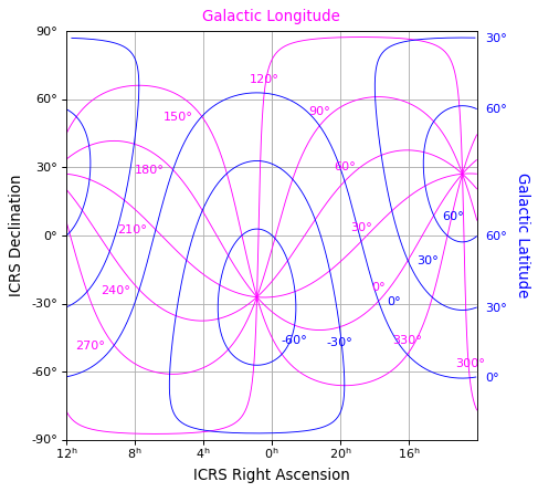
Interior ticks and tick labels
The default locations of ticks and tick labels for a WCSAxes rectangular plot are the edges of the frame.
It is now possible to place ticks or tick labels in the interior of the plot by using
add_tickable_gridline() to define a new “tickable” gridline.
Here is an example plot that uses this new functionality:
glon, glat = ax.get_coords_overlay('galactic')
glon.set_ticks(spacing=30*u.deg)
glat.set_ticks(spacing=30*u.deg)

glat.add_tickable_gridline('const-glat', 0*u.deg)
glon.add_tickable_gridline('const-glon', 0*u.deg)

glon.grid(color='magenta')
glon.set_ticks_visible(False)
glon.set_ticklabel_position(('const-glat',))
glon.set_ticklabel(color='magenta')
glon.set_axislabel('Galactic Longitude', color='magenta')

glat.grid(color='blue')
glat.set_ticks_visible(False)
glat.set_ticklabel_position(('const-glon', 'r'))
glat.set_ticklabel(color='blue')
glat.set_axislabel('Galactic Latitude', color='blue')

Support for tilde-prefixed paths
This release finishes adding support for tilde-prefixed paths, which began in
5.1. These are paths of the form ~/data/file.fits or
~<username>/data/file.fits. The single tilde refers to the current user’s
home directory, while a tilde followed by a valid username refers to that
user’s home directory (e.g. /home/<username> on Linux or
/Users/<username> on macOS). This syntax is common in command-line oriented
applications, especially on Unix-based systems. It serves as a convenient
shortcut, and it also allows code to be shared and run by multiple people
without having to update file paths if each person keeps data in the same
directory structure relative to their home directory.
This support has been added throughout the astropy.io module. This feature
is also supported within the I/O functionality of astropy.table and the
FITS-file functionality in astropy.nddata.
CCDData PSF Image representation
The NDData/CCDData objects now have a specific attribute for an image representation of the point spread function (PSF) at the image center.
This was added to support the Rubin Observatory/LSST alert packets, which will be distributed as CCDData objects.
Full change log
To see a detailed list of all changes in version v5.2, including changes in API, please see the Full Changelog.
Contributors to the v5.2 release
The people who have contributed to the code for this release are:
|
|
|
|
Where a * indicates that this release contains their first contribution to astropy.