Slicing Multidimensional Data

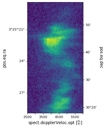
WCSAxes can either plot one or two dimensional data. If we have a dataset with higher dimensionality than the plot we want to make, we have to select which dimensions to use for the x or x and y axes of the plot. This example will show how to slice a FITS data cube and plot an image from it.

Slicing the WCS object

Like the example introduced in Initializing axes with world coordinates, we will read in the data using astropy.io.fits and parse the WCS information. The original FITS file can be downloaded from here.

import matplotlib.pyplot as plt
from astropy.wcs import WCS
from astropy.io import fits
from astropy.utils.data import get_pkg_data_filename
filename = get_pkg_data_filename('l1448/l1448_13co.fits')
hdu = fits.open(filename)[0]
wcs = WCS(hdu.header)
image_data = hdu.data

This is a three-dimensional dataset which you can check by looking at the header information by:

>>> hdu.header  
...
NAXIS = 3 /number of axes
CTYPE1  = 'RA---SFL'           /
CTYPE2  = 'DEC--SFL'           /
CTYPE3  = 'VELO-LSR'           /
...

The header keyword ‘NAXIS’ gives the number of dimensions of the dataset. The keywords ‘CTYPE1’, ‘CTYPE2’ and ‘CTYPE3’ give the data type of these dimensions to be right ascension, declination and velocity respectively.

We then instantiate the WCSAxes using the WCS object and select the slices we want to plot:

import matplotlib.pyplot as plt
ax = plt.subplot(projection=wcs, slices=(50, 'y', 'x'))

By setting slices=(50, 'y', 'x'), we have chosen to plot the second dimension on the y-axis and the third dimension on the x-axis. Even though we are not plotting the all the dimensions, we have to specify which slices to select for the dimensions that are not shown. In this example, we are not plotting the first dimension so we have selected the slice 50 to display. You can experiment with this by changing the selected slice and looking at how the plotted image changes.

Plotting the image

We then add the axes to the image and plot it using the method imshow().

ax.coords[2].set_ticklabel(exclude_overlapping=True)
ax.imshow(image_data[:, :, 50].transpose())

(png, svg, pdf)

Here, image_data is an ndarray object. In Numpy, the order of the axes is reversed so the first dimension in the FITS file appears last, the last dimension appears first and so on. Therefore the index passed to imshow() should be the same as passed to slices but in reversed order. We also need to transpose() image_data as we have reversed the dimensions plotted on the x and y axes in the slice.

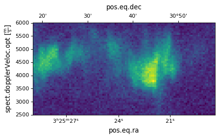
If we don’t want to reverse the dimensions plotted, we can simply do:

import matplotlib.pyplot as plt
ax = plt.subplot(projection=wcs, slices=(50, 'x', 'y'))
ax.imshow(image_data[:, :, 50])

(png, svg, pdf)

Plotting one dimensional data

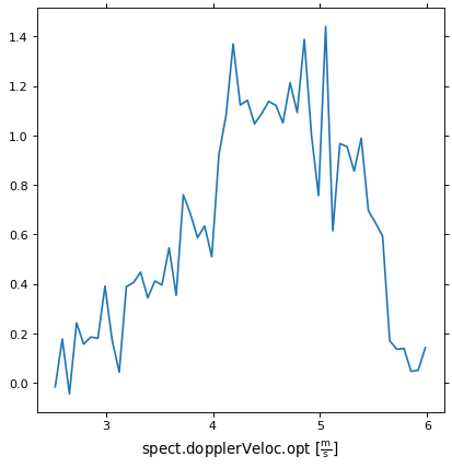
If we wanted to plot the spectral axes for one pixel we can do this by slicing down to one dimension.

import matplotlib.pyplot as plt
ax = plt.subplot(projection=wcs, slices=(50, 50, 'x'))

Here we have selected the 50 pixel in the first and second dimensions and will use the third dimension as our x axis.

We can now plot the spectral axis for this pixel. Note that we are plotting against pixel coordinates in the call to ax.plot, WCSAxes will display the world coordinates for us.

ax.plot(image_data[:, 50, 50])

As this is still a WCSAxes plot, we can set the display units for the x-axis

ra, dec, vel = ax.coords
vel.set_format_unit(u.km/u.s)

(png, svg, pdf)

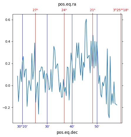
If we wanted to plot a one dimensional plot along a spatial dimension, i.e. intensity along a row in the image, WCSAxes defaults to displaying both the world coordinates for this plot. We can customise the colors and add grid lines for each of the spatial axes.

import matplotlib.pyplot as plt
ax = plt.subplot(projection=wcs, slices=(50, 'x', 0))

ax.plot(image_data[0, :, 50])

ra, dec, wave = ax.coords
ra.set_ticks(color="red")
ra.set_ticklabel(color="red")
ra.grid(color="red")

dec.set_ticks(color="blue")
dec.set_ticklabel(color="blue")
dec.grid(color="blue")

(png, svg, pdf)