Choosing Histogram Bins

The astropy.visualization module provides the hist() function, which is a generalization of matplotlib’s histogram function which allows for more flexible specification of histogram bins. For computing bins without the accompanying plot, see astropy.stats.histogram().

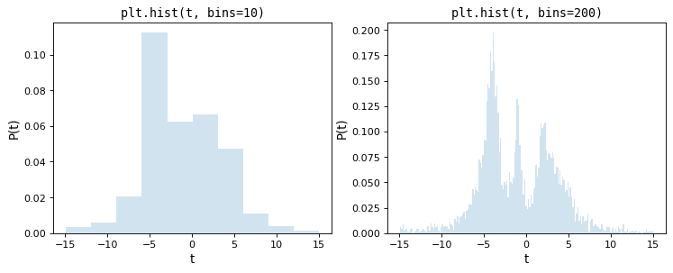
As a motivation for this, consider the following two histograms, which are constructed from the same underlying set of 5000 points, the first with matplotlib’s default of 10 bins, the second with an arbitrarily chosen 200 bins:

import numpy as np
import matplotlib.pyplot as plt

# generate some complicated data
rng = np.random.default_rng(0)
t = np.concatenate([-5 + 1.8 * rng.standard_cauchy(500),
                    -4 + 0.8 * rng.standard_cauchy(2000),
                    -1 + 0.3 * rng.standard_cauchy(500),
                    2 + 0.8 * rng.standard_cauchy(1000),
                    4 + 1.5 * rng.standard_cauchy(1000)])

# truncate to a reasonable range
t = t[(t > -15) & (t < 15)]

# draw histograms with two different bin widths
fig, ax = plt.subplots(1, 2, figsize=(10, 4))

fig.subplots_adjust(left=0.1, right=0.95, bottom=0.15)
for i, bins in enumerate([10, 200]):
    ax[i].hist(t, bins=bins, histtype='stepfilled', alpha=0.2, density=True)
    ax[i].set_xlabel('t')
    ax[i].set_ylabel('P(t)')
    ax[i].set_title(f'plt.hist(t, bins={bins})',
                    fontdict=dict(family='monospace'))

(png, svg, pdf)

Upon visual inspection, it is clear that each of these choices is suboptimal: with 10 bins, the fine structure of the data distribution is lost, while with 200 bins, heights of individual bins are affected by sampling error. The tried-and-true method employed by most scientists is a trial and error approach that attempts to find a suitable midpoint between these.

Astropy’s hist() function addresses this by providing several methods of automatically tuning the histogram bin size. It has a syntax identical to matplotlib’s plt.hist function, with the exception of the bins parameter, which allows specification of one of four different methods for automatic bin selection. These methods are implemented in astropy.stats.histogram(), which has a similar syntax to the np.histogram function.

Normal Reference Rules

The simplest methods of tuning the number of bins are the normal reference rules due to Scott (implemented in scott_bin_width()) and Freedman & Diaconis (implemented in freedman_bin_width()). These rules proceed by assuming the data is close to normally-distributed, and applying a rule-of-thumb intended to minimize the difference between the histogram and the underlying distribution of data.

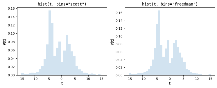
The following figure shows the results of these two rules on the above dataset:

import numpy as np
import matplotlib.pyplot as plt
from astropy.visualization import hist

# generate some complicated data
rng = np.random.default_rng(0)
t = np.concatenate([-5 + 1.8 * rng.standard_cauchy(500),
                    -4 + 0.8 * rng.standard_cauchy(2000),
                    -1 + 0.3 * rng.standard_cauchy(500),
                    2 + 0.8 * rng.standard_cauchy(1000),
                    4 + 1.5 * rng.standard_cauchy(1000)])

# truncate to a reasonable range
t = t[(t > -15) & (t < 15)]

# draw histograms with two different bin widths
fig, ax = plt.subplots(1, 2, figsize=(10, 4))

fig.subplots_adjust(left=0.1, right=0.95, bottom=0.15)
for i, bins in enumerate(['scott', 'freedman']):
    hist(t, bins=bins, ax=ax[i], histtype='stepfilled',
         alpha=0.2, density=True)
    ax[i].set_xlabel('t')
    ax[i].set_ylabel('P(t)')
    ax[i].set_title(f'hist(t, bins="{bins}")',
                    fontdict=dict(family='monospace'))

(png, svg, pdf)

As we can see, both of these rules of thumb choose an intermediate number of bins which provide a good trade-off between data representation and noise suppression.

Bayesian Models

Though rules-of-thumb like Scott’s rule and the Freedman-Diaconis rule are fast and convenient, their strong assumptions about the data make them suboptimal for more complicated distributions. Other methods of bin selection use fitness functions computed on the actual data to choose an optimal binning. Astropy implements two of these examples: Knuth’s rule (implemented in knuth_bin_width()) and Bayesian Blocks (implemented in bayesian_blocks()).

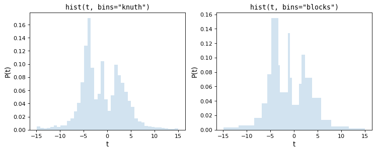
Knuth’s rule chooses a constant bin size which minimizes the error of the histogram’s approximation to the data, while the Bayesian Blocks uses a more flexible method which allows varying bin widths. Because both of these require the minimization of a cost function across the dataset, they are more computationally intensive than the rules-of-thumb mentioned above. Here are the results of these procedures for the above dataset:

import warnings
import numpy as np
import matplotlib.pyplot as plt
from astropy.visualization import hist

# generate some complicated data
rng = np.random.default_rng(0)
t = np.concatenate([-5 + 1.8 * rng.standard_cauchy(500),
                    -4 + 0.8 * rng.standard_cauchy(2000),
                    -1 + 0.3 * rng.standard_cauchy(500),
                    2 + 0.8 * rng.standard_cauchy(1000),
                    4 + 1.5 * rng.standard_cauchy(1000)])

# truncate to a reasonable range
t = t[(t > -15) & (t < 15)]

# draw histograms with two different bin widths
fig, ax = plt.subplots(1, 2, figsize=(10, 4))

fig.subplots_adjust(left=0.1, right=0.95, bottom=0.15)
for i, bins in enumerate(['knuth', 'blocks']):
    hist(t, bins=bins, ax=ax[i], histtype='stepfilled',
            alpha=0.2, density=True)
    ax[i].set_xlabel('t')
    ax[i].set_ylabel('P(t)')
    ax[i].set_title(f'hist(t, bins="{bins}")',
                    fontdict=dict(family='monospace'))

(png, svg, pdf)

Notice that both of these capture the shape of the distribution very accurately, and that the bins='blocks' panel selects bin widths which vary in width depending on the local structure in the data. Compared to standard defaults, these Bayesian optimization methods provide a much more principled means of choosing histogram binning.