Lomb-Scargle Periodograms

The Lomb-Scargle periodogram (after Lomb [1], and Scargle [2]) is a commonly used statistical tool designed to detect periodic signals in unevenly spaced observations. The LombScargle class is a unified interface to several implementations of the Lomb-Scargle periodogram, including a fast O[NlogN] implementation following the algorithm presented by Press & Rybicki [3].

The code here is adapted from the astroml package ([4], [5]) and the gatspy package ([6], [7]). For a detailed practical discussion of the Lomb-Scargle periodogram, with code examples based on astropy, see Understanding the Lomb-Scargle Periodogram [11], with associated code at https://github.com/jakevdp/PracticalLombScargle/.

Basic Usage

Note

All frequencies in LombScargle are not angular frequencies, but rather frequencies of oscillation (i.e., number of cycles per unit time).

The Lomb-Scargle periodogram is designed to detect periodic signals in unevenly spaced observations.

Example

To detect periodic signals in unevenly spaced observations, consider the following data:

>>> import numpy as np
>>> rand = np.random.default_rng(42)
>>> t = 100 * rand.random(100)
>>> y = np.sin(2 * np.pi * t) + 0.1 * rand.standard_normal(100)

These are 100 noisy measurements taken at irregular times, with a frequency of 1 cycle per unit time.

The Lomb-Scargle periodogram, evaluated at frequencies chosen automatically based on the input data, can be computed as follows using the LombScargle class:

>>> from astropy.timeseries import LombScargle
>>> frequency, power = LombScargle(t, y).autopower()

Plotting the result with Matplotlib gives:

>>> import matplotlib.pyplot as plt  
>>> plt.plot(frequency, power)       

(png, svg, pdf)

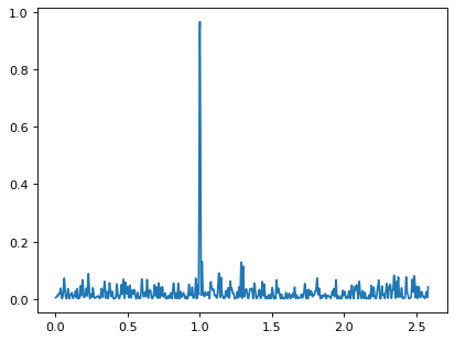
The periodogram shows a clear spike at a frequency of 1 cycle per unit time, as we would expect from the data we constructed.

Measurement Uncertainties

The LombScargle interface can also handle data with measurement uncertainties.

Example

If all uncertainties are the same, you can pass a scalar:

>>> dy = 0.1
>>> frequency, power = LombScargle(t, y, dy).autopower()

If uncertainties vary from observation to observation, you can pass them as an array:

>>> dy = 0.1 * (1 + rand.random(100))
>>> y = np.sin(2 * np.pi * t) + dy * rand.standard_normal(100)
>>> frequency, power = LombScargle(t, y, dy).autopower()

Gaussian uncertainties are assumed, and dy here specifies the standard deviation (not the variance).

Periodograms and Units

The LombScargle interface properly handles Quantity objects with units attached, and will validate the inputs to make sure units are appropriate.

Example

To use the LombScargle for Quantity objects with units attached:

>>> import astropy.units as u
>>> t_days = t * u.day
>>> y_mags = y * u.mag
>>> dy_mags = y * u.mag
>>> frequency, power = LombScargle(t_days, y_mags, dy_mags).autopower()
>>> frequency.unit
Unit("1 / d")
>>> power.unit
Unit(dimensionless)

We see that the output is dimensionless, which is always the case for the standard normalized periodogram (for more on normalizations, see Periodogram Normalizations below). If you include arguments to autopower such as minimum_frequency or maximum_frequency, make sure to specify units as well:

>>> frequency, power = LombScargle(t_days, y_mags, dy_mags).autopower(minimum_frequency=1e-5*u.Hz)

Specifying the Frequency

With the autopower() method used above, a heuristic is applied to select a suitable frequency grid. By default, the heuristic assumes that the width of peaks is inversely proportional to the observation baseline, and that the maximum frequency is a factor of five larger than the so-called “average Nyquist frequency,” with computation based on the average observation spacing.

This heuristic is not universally useful, as the frequencies probed by irregularly sampled data can be much higher than the average Nyquist frequency. For this reason, the heuristic can be tuned through keywords passed to the autopower() method.

Example

To tune the heuristic using keywords passed to the autopower() method:

>>> frequency, power = LombScargle(t, y, dy).autopower(nyquist_factor=2)
>>> len(frequency), frequency.min(), frequency.max()  
(500, 0.0010327803641893758, 1.0317475838251864)

Here the highest frequency is two times the average Nyquist frequency. If we increase the nyquist_factor, we can probe higher frequencies:

>>> frequency, power = LombScargle(t, y, dy).autopower(nyquist_factor=10)
>>> len(frequency), frequency.min(), frequency.max()  
(2500, 0.0010327803641893758, 5.16286904058269)

Alternatively, we can use the power() method to evaluate the periodogram at a user-specified set of frequencies:

>>> frequency = np.linspace(0.5, 1.5, 1000)
>>> power = LombScargle(t, y, dy).power(frequency)

Note that the fastest Lomb-Scargle implementation requires regularly spaced frequencies; if frequencies are irregularly spaced, a slower method will be used instead.

Frequency Grid Spacing

One common issue with user-specified frequencies is inadvertently choosing too coarse a grid, such that significant peaks lie between grid points and are missed entirely.

Example

Imagine you chose to evaluate your periodogram at 100 points:

>>> frequency = np.linspace(0.1, 1.9, 100)
>>> power = LombScargle(t, y, dy).power(frequency)
>>> plt.plot(frequency, power)   

(png, svg, pdf)

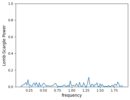
From this plot alone, you might conclude that no clear periodic signal exists in the data. But this conclusion is in error: there is in fact a strong periodic signal, but the periodogram peak falls in the gap between the chosen grid points!

A more reliable approach is to use the frequency heuristic to decide on the appropriate grid spacing, optionally passing a minimum and maximum frequency to the autopower() method:

>>> frequency, power = LombScargle(t, y, dy).autopower(minimum_frequency=0.1,
...                                                    maximum_frequency=1.9)
>>> len(frequency)
872
>>> plt.plot(frequency, power)   

(png, svg, pdf)

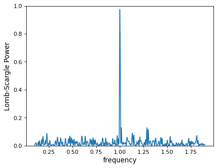
With a finer grid (here 884 points between 0.1 and 1.9), it is clear that there is a very strong periodic signal in the data.

By default, the heuristic aims to have roughly five grid points across each significant periodogram peak; this can be increased by changing the samples_per_peak argument:

>>> frequency, power = LombScargle(t, y, dy).autopower(minimum_frequency=0.1,
...                                                    maximum_frequency=1.9,
...                                                    samples_per_peak=10)
>>> len(frequency)
1744

Keep in mind that the width of the peak scales inversely with the baseline of the observations (i.e., the difference between the maximum and minimum time), and the required number of grid points will scale linearly with the size of the baseline.

The Lomb-Scargle Model

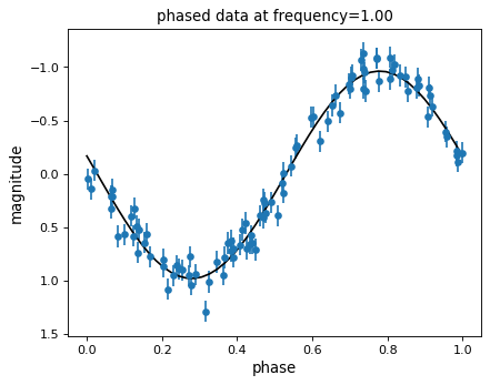
The Lomb-Scargle periodogram fits a sinusoidal model to the data at each frequency, with a larger power reflecting a better fit. With this in mind, it is often helpful to plot the best-fit sinusoid over the phased data.

Example

This best-fit sinusoid can be computed using the model() method of the LombScargle object:

>>> best_frequency = frequency[np.argmax(power)]
>>> t_fit = np.linspace(0, 1)
>>> ls = LombScargle(t, y, dy)
>>> y_fit = ls.model(t_fit, best_frequency)

We can then phase the data and plot the Lomb-Scargle model fit:

(png, svg, pdf)

The best-fit model parameters can be computed with the model_parameters() method of the LombScargle object at a given frequency:

>>> theta = ls.model_parameters(best_frequency)
>>> theta.round(2)
array([-0.01,  0.99,  0.11])

These parameters \(\vec{\theta}\) are fit using the following model:

\[y(t; f, \vec{\theta}) = \theta_0 + \sum_{n=1}^{\tt nterms} [\theta_{2n-1}\sin(2\pi n f t) + \theta_{2n}\cos(2\pi n f t)]\]

The model can be constructed from these parameters by computing the associated offset(), which accounts for the pre-centering of data (i.e., the center_data argument), and design_matrix(), which computes the sine and cosine terms for you:

>>> offset = ls.offset()
>>> design_matrix = ls.design_matrix(best_frequency, t_fit)
>>> np.allclose(y_fit, offset + design_matrix.dot(theta))
True

Additional Arguments

On initialization, LombScargle takes a few additional arguments which control the model for the data:

• center_data (True by default) controls whether the y values are pre-centered before the algorithm fits the data. The only time it is really warranted to change the default is if you are computing the periodogram of a sequence of constant values to, for example, estimate the window power spectrum for a series of observations.

• fit_mean (True by default) controls whether the model fits for the mean of the data, rather than assuming the mean is zero. When fit_mean=True, the periodogram is more robust than the original Lomb-Scargle formalism, particularly in the case of smaller sample sizes and/or data with nontrivial selection bias. In the literature, this model has variously been called the date-compensated discrete Fourier transform, the floating-mean periodogram, the generalized Lomb-Scargle method, and likely other names as well.

• nterms (1 by default) controls how many Fourier terms are used in the model. As seen above, the standard Lomb-Scargle periodogram is equivalent to a single-term sinusoidal fit to the data at each frequency; the generalization is to expand this to a truncated Fourier series with multiple frequencies. While this can be very useful in some cases, in others the additional model complexity can lead to spurious periodogram peaks that outweigh the benefit of the more flexible model.

Periodogram Normalizations

There are several normalizations of the Lomb-Scargle periodogram found in the literature. LombScargle makes four options available via the normalization argument: normalization='standard' (the default), normalization='model', normalization='log', and normalization='psd'. These normalizations can be thought of in terms of least-squares fits around a constant reference model \(M_{ref}\) and a periodic model \(M(f)\) at each frequency, with best-fit sum of residuals that we will denote by \(\chi^2_{ref}\) and \(\chi^2(f)\) respectively.

Standard Normalization

The default, the standard normalized periodogram is normalized by the residuals of the data around the constant reference model:

\[P_{standard}(f) = \frac{\chi^2_{ref} - \chi^2(f)}{\chi^2_{ref}}\]

This form of the normalization (normalization='standard') is the default choice used in LombScargle. The resulting power P is a dimensionless quantity that lies in the range 0 ≤ P ≤ 1.

Model Normalization

Alternatively, the periodogram is sometimes normalized instead by the residuals around the periodic model:

\[P_{model}(f) = \frac{\chi^2_{ref} - \chi^2(f)}{\chi^2(f)}\]

This form of the normalization can be specified with normalization='model'. As above, the resulting power is a dimensionless quantity that lies in the range 0 ≤ P ≤ ∞.

Logarithmic Normalization

Another form of normalization is to scale the periodogram logarithmically:

\[P_{log}(f) = \log \frac{\chi^2_{ref}}{\chi^2(f)}\]

This normalization can be specified with normalization='log', and the resulting power is a dimensionless quantity in the range 0 ≤ P ≤ ∞.

PSD Normalization (Unnormalized)

Finally, it is sometimes useful to compute an unnormalized periodogram (normalization='psd'):

\[P_{psd}(f) = \frac{1}{2}\left(\chi^2_{ref} - \chi^2(f)\right)\]

Which, in the case of no-uncertainty, will have units y.unit ** 2. This normalization is constructed to be comparable to the standard Fourier power spectral density (PSD):

>>> ls = LombScargle(t_days, y_mags, normalization='psd')
>>> frequency, power = ls.autopower()
>>> power.unit
Unit("mag2")

Note, however, that the normalization='psd' result only has these units if uncertainties are not specified. In the presence of uncertainties, even the unnormalized PSD periodogram will be dimensionless; this is due to the scaling of data by uncertainty within the Lomb-Scargle computation:

>>> # with uncertainties, PSD power is unitless
>>> ls = LombScargle(t_days, y_mags, dy_mags, normalization='psd')
>>> frequency, power = ls.autopower()
>>> power.unit
Unit(dimensionless)

The equivalence of the PSD-normalized periodogram and the Fourier PSD in the unnormalized, no-uncertainty case can be confirmed by comparing results directly for uniformly sampled inputs.

We will first define a convenience function to compute the basic Fourier periodogram for uniformly sampled quantities:

>>> def fourier_periodogram(t, y):
...     N = len(t)
...     frequency = np.fft.fftfreq(N, t[1] - t[0])
...     y_fft = np.fft.fft(y.value) * y.unit
...     positive = (frequency > 0)
...     return frequency[positive], (1. / N) * abs(y_fft[positive]) ** 2

Next we compute the two versions of the PSD from uniformly sampled data:

>>> t_days = np.arange(100) * u.day
>>> y_mags = rand.standard_normal(100) * u.mag
>>> frequency, PSD_fourier = fourier_periodogram(t_days, y_mags)
>>> ls = LombScargle(t_days, y_mags, normalization='psd')
>>> PSD_LS = ls.power(frequency)

Examining the results, we see that the two outputs match:

>>> u.allclose(PSD_fourier, PSD_LS)
True

This equivalence is one reason that the Lomb-Scargle periodogram is considered to be an extension of the Fourier PSD.

For more information on the statistical properties of these normalizations, see, for example, Baluev 2008 [8].

Peak Significance and False Alarm Probabilities

Note

Interpretation of Lomb-Scargle peak significance via false alarm probabilities is a subtle subject, and the quantities computed below are commonly misinterpreted or misused. For a detailed discussion of periodogram peak significance, see [11].

When using the Lomb-Scargle periodogram to decide whether a signal contains a periodic component, an important consideration is the significance of the periodogram peak. This significance is usually expressed in terms of a false alarm probability, which encodes the probability of measuring a peak of a given height (or higher) conditioned on the assumption that the data consists of Gaussian noise with no periodic component.

Example

To use the Lomb-Scargle periodogram to decide if our signal contains a periodic component, we can start by simulating 60 observations of a sine wave with noise:

>>> t = 100 * rand.random(60)
>>> dy = 1.0
>>> y = np.sin(2 * np.pi * t) + dy * rand.standard_normal(60)
>>> ls = LombScargle(t, y, dy)
>>> freq, power = ls.autopower()
>>> print(power.max())  
0.29154492887882927

The peak of the periodogram has a value of 0.33, but how significant is this peak? We can address this question using the false_alarm_probability() method:

>>> ls.false_alarm_probability(power.max())  
0.028959671719328808

What this tells us is that under the assumption that there is no periodic signal in the data, we will observe a peak this high or higher approximately 0.4% of the time, which gives a strong indication that a periodic signal is present in the data.

Note

Users must interpret this probability carefully: it is a measurement conditioned on the assumption of the null hypothesis of no signal; in symbols, you might write \(P({\rm data} \mid {\rm noise-only})\).

Although it may seem like this quantity could be interpreted with a statement such as “there is an 0.4% chance that this data is noise only,” this is not a correct statement; in symbols, this statement describes the quantity \(P({\rm noise-only} \mid {\rm data})\), and in general \(P(A\mid B) \ne P(B\mid A)\).

See [11] for a more detailed discussion of such caveats.

We might also wish to compute the required peak height to attain any given false alarm probability, which can be done with the false_alarm_level() method:

>>> probabilities = [0.1, 0.05, 0.01]
>>> ls.false_alarm_level(probabilities)  
array([0.25681381, 0.27663466, 0.31928202])

This tells us that to attain a 10% false alarm probability requires the highest periodogram peak to be approximately 0.25; 5% requires 0.27, and 1% requires 0.32.

False Alarm Approximations

Although the false alarm probability at any particular frequency is analytically computable, there is no closed-form analytic expression for the more relevant quantity of the false alarm level of the highest peak in a particular periodogram. This must be either determined through bootstrap simulations, or approximated by various means.

astropy provides four options for approximating the false alarm probability, which can be chosen using the method keyword:

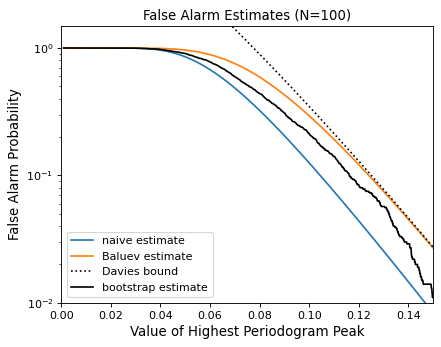
• method="baluev" (the default) implements the approximation proposed by Baluev 2008 [8], which employs extreme value statistics to compute an upper bound of the false alarm probability for the alias-free case. Experiments show that the bound is also useful even for highly aliased observing patterns.

>>> ls.false_alarm_probability(power.max(), method='baluev')  
0.028959671719328808

• method="bootstrap" implements a bootstrap simulation: effectively it computes many Lomb-Scargle periodograms on simulated data at the same observation times. The bootstrap approach can very accurately determine the false alarm probability, but is very computationally expensive. To estimate the level corresponding to a false alarm probability \(P_{false}\), it requires on order \(n_{boot} \approx 10/P_{false}\) individual periodograms to be computed for the dataset.

>>> ls.false_alarm_probability(power.max(), method='bootstrap')  
0.0030000000000000027

• method="davies" is related to the Baluev method, but loses accuracy at large false alarm probabilities.

>>> ls.false_alarm_probability(power.max(), method='davies')  
0.029387277355227746

• method="naive" is a basic method based on the assumption that well-separated areas in the periodogram are independent. In general, it provides a very poor estimate of the false alarm probability and should not be used in practice, but is included for completeness.

>>> ls.false_alarm_probability(power.max(), method='naive')  
0.00810080828660202

The following figure compares these false alarm estimates at a range of peak heights for 100 observations with a heavily aliased observing pattern:

(png, svg, pdf)

In general, users should use the bootstrap approach when computationally feasible, and the Baluev approach otherwise.

In all of this, it is important to keep in mind a few caveats:

• False alarm probabilities are computed relative to a particular set of observing times, and a particular choice of frequency grid.

• False alarm probabilities are conditioned upon the null hypothesis of data with no periodic component, and in particular say nothing quantitative about whether the data are actually consistent with a periodic model.

• False alarm probabilities are not related to the question of whether the highest peak in a periodogram is the correct peak, and in particular are not especially useful in the case of observations with a strong aliasing pattern.

For a detailed discussion of these caveats and others when computing and interpreting false alarm probabilities, please refer to [11].

Periodogram Algorithms

The LombScargle class makes available several complementary implementations of the Lomb-Scargle periodogram, which can be selected using the method keyword of the Lomb-Scargle power. By design all methods will return the same results (some approximate), and each has its advantages and disadvantages.

For example, to compute a periodogram using the Fast Chi-squared method of Palmer (2009) [9], you can specify method='fastchi2':

>>> frequency, power = LombScargle(t, y).autopower(method='fastchi2')

There are currently six methods available in the package:

method='auto'

The auto method is the default, and will attempt to select the best option from the following methods using heuristics driven by the input data.

method='slow'

The slow method is a pure Python implementation of the original Lomb-Scargle periodogram ([1], [2]), enhanced to account for observational noise, and to allow a floating mean (sometimes called the generalized periodogram; see [10]). The method is not particularly fast, scaling approximately as \(O[NM]\) for \(N\) data points and \(M\) frequencies.

method='cython'

The cython method is a Cython implementation of the same algorithm used for method='slow'. It is slightly faster than the pure Python implementation, but much more memory-efficient as the size of the inputs grow. The computational scaling is approximately \(O[NM]\) for \(N\) data points and \(M\) frequencies.

method='scipy'

The scipy method wraps the C implementation of the original Lomb-Scargle periodogram which is available in scipy.signal.lombscargle(). This is slightly faster than the slow method, but does not allow for errors in data or extensions such as the floating mean. The scaling is approximately \(O[NM]\) for \(N\) data points and \(M\) frequencies.

method='fast'

The fast method is a pure Python implementation of the fast periodogram of Press & Rybicki [3]. It uses an extrapolation approach to approximate the periodogram frequencies using a fast Fourier transform. As with the slow method, it can handle data errors and floating mean. The scaling is approximately \(O[N\log M]\) for \(N\) data points and \(M\) frequencies. The fast algorithm trades accuracy for speed, and produces a close approximation to the true periodogram. In particular, you may observe powers less than zero in some cases.

method='chi2'

The chi2 method is a pure Python implementation based on matrix algebra (see [7]). It utilizes the fact that the Lomb-Scargle periodogram at each frequency is equivalent to the least-squares fit of a sinusoid to the data. The advantage of the chi2 method is that it allows extensions of the periodogram to multiple Fourier terms, specified by the nterms parameter. For the standard problem, it is slightly slower than method='slow' and scales as \(O[n_fNM]\) for \(N\) data points, \(M\) frequencies, and \(n_f\) Fourier terms.

method='fastchi2'

The Fast Chi-squared method of Palmer (2009) [9] is equivalent to the chi2 method, but the matrices are constructed using an FFT-based approach similar to that of the fast method. The result is a relatively efficient periodogram (though not nearly as efficient as the fast method) which can be extended to multiple terms. The scaling is approximately \(O[n_f(M + N\log M)]\) for \(N\) data points, \(M\) frequencies, and \(n_f\) Fourier terms.

Summary

The following table summarizes the features of the above algorithms:

Method	Computational Scaling	Observational Uncertainties	Bias Term (Floating Mean)	Multiple Terms
"slow"	\(O[NM]\)	Yes	Yes	No
"cython"	\(O[NM]\)	Yes	Yes	No
"scipy"	\(O[NM]\)	No	No	No
"fast"	\(O[N\log M]\)	Yes	Yes	No
"chi2"	\(O[n_fNM]\)	Yes	Yes	Yes
"fastchi2"	\(O[n_f(M + N\log M)]\)	Yes	Yes	Yes

In the Computational Scaling column, \(N\) is the number of data points, \(M\) is the number of frequencies, and \(n_f\) is the number of Fourier terms for a multi-term fit.

RR Lyrae Example

An example of computing the periodogram for a more realistic dataset is shown in the following figure. The data here consists of 50 nightly observations of a simulated RR Lyrae-like variable star, with a lightcurve shape that is more complicated than a simple sine wave:

(png, svg, pdf)

The dotted line shows the periodogram level corresponding to a maximum peak false alarm probability of 1%. This example demonstrates that for irregularly sampled data, the Lomb-Scargle periodogram can be sensitive to frequencies higher than the average Nyquist frequency: the above data are sampled at an average rate of roughly one observation per night, and the periodogram relatively cleanly reveals the true period of 0.41 days.

Still, the periodogram has many spurious peaks, which are due to several factors:

1. Errors in observations lead to leakage of power from the true peaks.

2. The signal is not a perfect sinusoid, so additional peaks can indicate higher frequency components in the signal.

3. The observations take place only at night, meaning that the survey window has non-negligible power at a frequency of 1 cycle per day. Thus we expect aliases to appear at \(f_{\rm alias} = f_{\rm true} + n f_{\rm window}\) for integer values of \(n\). With a true period of 0.41 days and a 1-day signal in the observing window, the \(n=+1\) and \(n=-1\) aliases to lie at periods of 0.29 and 0.69 days, respectively: these aliases are prominent in the above plot.

The interaction of these effects means that in practice there is no absolute guarantee that the highest peak corresponds to the best frequency, and results must be interpreted carefully. For a detailed discussion of these effects, see [11].

Literature References

[1] (1,2)

Lomb, N.R. Least-squares frequency analysis of unequally spaced data. Ap&SS 39 pp. 447-462 (1976)

[2] (1,2)

Scargle, J. D. Studies in astronomical time series analysis. II - Statistical aspects of spectral analysis of unevenly spaced data. ApJ 1:263 pp. 835-853 (1982)

[3] (1,2)

Press W.H. and Rybicki, G.B, Fast algorithm for spectral analysis of unevenly sampled data. ApJ 1:338, p. 277 (1989)

[4]

Vanderplas, J., Connolly, A. Ivezic, Z. & Gray, A. Introduction to astroML: Machine learning for astrophysics. Proceedings of the Conference on Intelligent Data Understanding (2012)

[5]

Vanderplas, J., Connolly, A. Ivezic, Z. & Gray, A. Statistics, Data Mining and Machine Learning in Astronomy. Princeton Press (2014)}

[6]

VanderPlas, J. Gatspy: General Tools for Astronomical Time Series in Python (2015) https://zenodo.org/record/14833

[7] (1,2)

VanderPlas, J. & Ivezic, Z. Periodograms for Multiband Astronomical Time Series. ApJ 812.1:18 (2015)

[8] (1,2)

Baluev, R.V. Assessing Statistical Significance of Periodogram Peaks MNRAS 385, 1279 (2008)

[9] (1,2)

Palmer, D. A Fast Chi-squared Technique for Period Search of Irregularly Sampled Data. ApJ 695.1:496 (2009)

[10]

Zechmeister, M. and Kurster, M. The generalised Lomb-Scargle periodogram. A new formalism for the floating-mean and Keplerian periodograms, A&A 496, 577-584 (2009)

[11] (1,2,3,4,5)

VanderPlas, J. Understanding the Lomb-Scargle Periodogram ApJS 236.1:16 (2018) https://ui.adsabs.harvard.edu/abs/2018ApJS..236…16V