Manipulation and Analysis of Time Series
Combining Time Series
The vstack() and hstack() functions
from the astropy.table module can be used to stack time series in
different ways.
Examples
Time series can be stacked “vertically” or row-wise using the
vstack() function (although note that sampled time
series cannot be combined with binned time series and vice versa):
>>> from astropy.table import vstack
>>> from astropy import units as u
>>> from astropy.timeseries import TimeSeries
>>> ts_a = TimeSeries(time_start='2016-03-22T12:30:31',
...                   time_delta=3 * u.s,
...                   data={'flux': [1, 4, 5, 3, 2] * u.mJy})
>>> ts_b = TimeSeries(time_start='2016-03-22T12:50:31',
...                   time_delta=3 * u.s,
...                   data={'flux': [4, 3, 1, 2, 3] * u.mJy})
>>> ts_ab = vstack([ts_a, ts_b])
>>> ts_ab
<TimeSeries length=10>
          time            flux
                          mJy
          Time          float64
----------------------- -------
2016-03-22T12:30:31.000     1.0
2016-03-22T12:30:34.000     4.0
2016-03-22T12:30:37.000     5.0
2016-03-22T12:30:40.000     3.0
2016-03-22T12:30:43.000     2.0
2016-03-22T12:50:31.000     4.0
2016-03-22T12:50:34.000     3.0
2016-03-22T12:50:37.000     1.0
2016-03-22T12:50:40.000     2.0
2016-03-22T12:50:43.000     3.0
Note that vstack() does not automatically sort, nor get rid
of duplicates — this is something you would need to do explicitly afterwards.
Time series can also be combined “horizontally” or column-wise with other tables
using the hstack() function, though these should not be
time series (as having multiple time columns would be confusing):
>>> from astropy.table import Table, hstack
>>> data = Table(data={'temperature': [40., 41., 40., 39., 30.] * u.K})
>>> ts_a_data = hstack([ts_a, data])
>>> ts_a_data
<TimeSeries length=5>
          time            flux  temperature
                          mJy          K
          Time          float64    float64
----------------------- ------- -----------
2016-03-22T12:30:31.000     1.0        40.0
2016-03-22T12:30:34.000     4.0        41.0
2016-03-22T12:30:37.000     5.0        40.0
2016-03-22T12:30:40.000     3.0        39.0
2016-03-22T12:30:43.000     2.0        30.0
Sorting Time Series
Sorting time series in place can be done using the
sort() method, as for Table:
>>> ts = TimeSeries(time_start='2016-03-22T12:30:31',
...                 time_delta=3 * u.s,
...                 data={'flux': [1., 4., 5., 3., 2.]})
>>> ts
<TimeSeries length=5>
          time            flux
          Time          float64
----------------------- -------
2016-03-22T12:30:31.000     1.0
2016-03-22T12:30:34.000     4.0
2016-03-22T12:30:37.000     5.0
2016-03-22T12:30:40.000     3.0
2016-03-22T12:30:43.000     2.0
>>> ts.sort('flux')
>>> ts
<TimeSeries length=5>
          time            flux
          Time          float64
----------------------- -------
2016-03-22T12:30:31.000     1.0
2016-03-22T12:30:43.000     2.0
2016-03-22T12:30:40.000     3.0
2016-03-22T12:30:34.000     4.0
2016-03-22T12:30:37.000     5.0
Resampling
We provide a aggregate_downsample() function
that can be used to bin values from a time series into equal-size or uneven bins,
and contiguous and non-contiguous bins, using a custom function (mean, median, etc.).
This operation returns a BinnedTimeSeries. Note that this is a basic function in
the sense that it does not, for example, know how to treat columns with uncertainties
differently from other values, and it will blindly apply the custom function
specified to all columns.
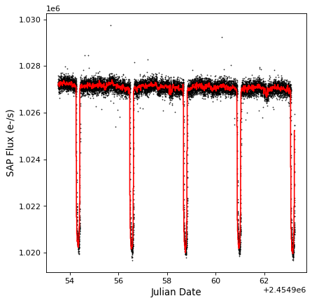
Example
The following example shows how to use
aggregate_downsample() to bin a light curve from the
Kepler mission into 20 minute contiguous bins using a median function. First,
we read in the data using:
from astropy.timeseries import TimeSeries
from astropy.utils.data import get_pkg_data_filename
example_data = get_pkg_data_filename('timeseries/kplr010666592-2009131110544_slc.fits')
kepler = TimeSeries.read(example_data, format='kepler.fits')
(See Reading and Writing Time Series for more details about reading in data). We can then downsample using:
import numpy as np
from astropy import units as u
from astropy.timeseries import aggregate_downsample
kepler_binned = aggregate_downsample(kepler, time_bin_size=20 * u.min, aggregate_func=np.nanmedian)
We can take a look at the results:
import matplotlib.pyplot as plt
plt.plot(kepler.time.jd, kepler['sap_flux'], 'k.', markersize=1)
plt.plot(kepler_binned.time_bin_start.jd, kepler_binned['sap_flux'], 'r-', drawstyle='steps-pre')
plt.xlabel('Julian Date')
plt.ylabel('SAP Flux (e-/s)')
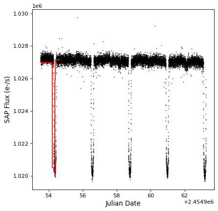
The aggregate_downsample() can also be used
to bin the light curve into custom bins. The following example shows
the case of uneven-size contiguous bins:
kepler_binned = aggregate_downsample(kepler, time_bin_size=[1000, 125, 80, 25, 150, 210, 273] * u.min,
                                     aggregate_func=np.nanmedian)

plt.plot(kepler.time.jd, kepler['sap_flux'], 'k.', markersize=1)
plt.plot(kepler_binned.time_bin_start.jd, kepler_binned['sap_flux'], 'r-', drawstyle='steps-pre')
plt.xlabel('Julian Date')
plt.ylabel('SAP Flux (e-/s)')
To learn more about the custom binning functionality in
aggregate_downsample(), see
Initializing a Binned Time Series.
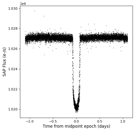
Folding
The TimeSeries class has a
fold() method that can be used to
return a new time series with a relative and folded time axis. This method
takes the period as a Quantity, and optionally takes
an epoch as a Time, which defines a zero time offset:
kepler_folded = kepler.fold(period=2.2 * u.day, epoch_time='2009-05-02T20:53:40')

plt.plot(kepler_folded.time.jd, kepler_folded['sap_flux'], 'k.', markersize=1)
plt.xlabel('Time from midpoint epoch (days)')
plt.ylabel('SAP Flux (e-/s)')

Note that in this example we happened to know the period and midpoint from a previous periodogram analysis. See the example in Time Series (astropy.timeseries) for how you might do this.
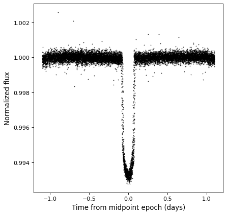
Arithmetic
Since TimeSeries objects are subclasses of Table, they naturally support
arithmetic on any of the data columns. As an example, we can take the folded
Kepler time series we have seen in previous examples, and normalize it to the
sigma-clipped median value.
from astropy.stats import sigma_clipped_stats

mean, median, stddev = sigma_clipped_stats(kepler_folded['sap_flux'])

kepler_folded['sap_flux_norm'] = kepler_folded['sap_flux'] / median

plt.plot(kepler_folded.time.jd, kepler_folded['sap_flux_norm'], 'k.', markersize=1)
plt.xlabel('Time from midpoint epoch (days)')
plt.ylabel('Normalized flux')