Fitting Model Sets
Astropy model sets let you fit the same (linear) model to lots of independent data sets. It solves the linear equations simultaneously, so can avoid looping. But getting the data into the right shape can be a bit tricky.
The time savings could be worth the effort. In the example below, if we change the width*height of the data cube to 500*500 it takes 140 ms on a 2015 MacBook Pro to fit the models using model sets. Doing the same fit by looping over the 500*500 models takes 1.5 minutes, more than 600 times slower.
In the example below, we create a 3D data cube where the first dimension is a ramp – for example as from non-destructive readouts of an IR detector. So each pixel has a depth along a time axis, and flux that results a total number of counts that is increasing with time. We will be fitting a 1D polynomial vs. time to estimate the flux in counts/second (the slope of the fit). We will use just a small image of 3 rows by 4 columns, with a depth of 10 non-destructive reads.
First, import the necessary libraries:
>>> import numpy as np
>>> rng = np.random.default_rng(seed=12345)
>>> from astropy.modeling import models, fitting
>>> depth, width, height = 10, 3, 4  # Time is along the depth axis
>>> t = np.arange(depth, dtype=np.float64)*10.  # e.g. readouts every 10 seconds
The number of counts in neach pixel is flux*time with the addition of some Gaussian noise:
>>> fluxes = np.arange(1. * width * height).reshape(width, height)
>>> image = fluxes[np.newaxis, :, :] * t[:, np.newaxis, np.newaxis]
>>> image += rng.normal(0., image*0.05, size=image.shape)  # Add noise
>>> image.shape
(10, 3, 4)
Create the models and the fitter. We need N=width*height instances of the same linear, parametric model (model sets currently only work with linear models and fitters):
>>> N = width * height
>>> line = models.Polynomial1D(degree=1, n_models=N)
>>> fit = fitting.LinearLSQFitter()
>>> print(f"We created {len(line)} models")
We created 12 models
We need to get the data to be fit into the right shape. It’s not possible to just feed
the 3D data cube. In this case, the time axis can be one dimensional.
The fluxes have to be organized into an array that is of shape width*height,depth – in
other words, we are reshaping to flatten last two axes and transposing to put them first:
>>> pixels = image.reshape((depth, width*height))
>>> y = pixels.T
>>> print("x axis is one dimensional: ",t.shape)
x axis is one dimensional:  (10,)
>>> print("y axis is two dimensional, N by len(x): ", y.shape)
y axis is two dimensional, N by len(x):  (12, 10)
Fit the model. It fits the N models simultaneously:
>>> new_model = fit(line, x=t, y=y)
>>> print(f"We fit {len(new_model)} models")
We fit 12 models
Fill an array with values computed from the best fit and reshape it to match the original:
>>> best_fit = new_model(t, model_set_axis=False).T.reshape((depth, height, width))
>>> print("We reshaped the best fit to dimensions: ", best_fit.shape)
We reshaped the best fit to dimensions:  (10, 4, 3)
Now inspect the model:
>>> print(new_model)
Model: Polynomial1D
Inputs: ('x',)
Outputs: ('y',)
Model set size: 12
Degree: 1
Parameters:
             c0                 c1
    ------------------- ------------------
                    0.0                0.0
     0.7435257251672668 0.9788645710692938
    -2.9342067207465647  2.038294797728997
     -4.258776494573452 3.1951399579785678
      2.364390501364263 3.9973270072631104
      2.161531512810536  4.939542306192216
     3.9930177540418823  5.967786182181591
     -6.825657765397985 7.2680615507233215
     -6.675677073701012  8.321048309260679
     -11.91115500400788  9.025794163936956
     -4.123655771677581  9.938564642105128
    -0.7256700167533869 10.989896974949136

>>> print("The new_model has a param_sets attribute with shape: ",new_model.param_sets.shape)
The new_model has a param_sets attribute with shape:  (2, 12)

>>> print(f"And values that are the best-fit parameters for each pixel:\n{new_model.param_sets}")
And values that are the best-fit parameters for each pixel:
[[  0.           0.74352573  -2.93420672  -4.25877649   2.3643905
    2.16153151   3.99301775  -6.82565777  -6.67567707 -11.911155
   -4.12365577  -0.72567002]
 [  0.           0.97886457   2.0382948    3.19513996   3.99732701
    4.93954231   5.96778618   7.26806155   8.32104831   9.02579416
    9.93856464  10.98989697]]
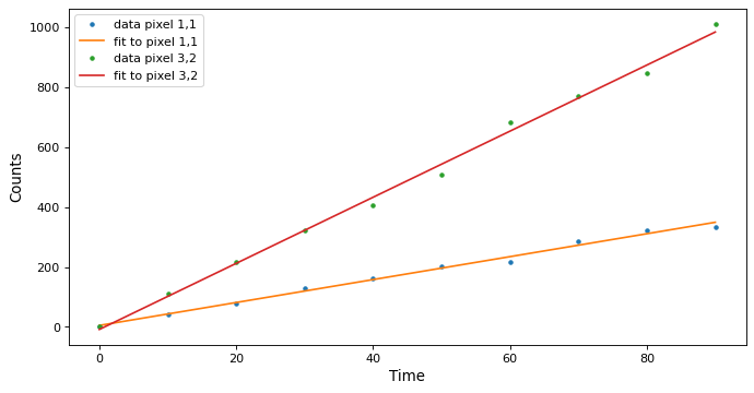
Plot the fit along a couple of pixels:
>>> def plotramp(t, image, best_fit, row, col):
...     plt.plot(t, image[:, row, col], '.', label=f'data pixel {row},{col}')
...     plt.plot(t, best_fit[:, row, col], '-', label=f'fit to pixel {row},{col}')
...     plt.xlabel('Time')
...     plt.ylabel('Counts')
...     plt.legend(loc='upper left')
>>> fig = plt.figure(figsize=(10, 5))
>>> plotramp(t, image, best_fit, 1, 1)
>>> plotramp(t, image, best_fit, 2, 1)
The data and the best fit model are shown together on one plot.
