Fitting with constraints
fitting support constraints, however, different fitters support
different types of constraints. The supported_constraints
attribute shows the type of constraints supported by a specific fitter:
>>> from astropy.modeling import fitting
>>> fitting.LinearLSQFitter.supported_constraints
['fixed']
>>> fitting.LevMarLSQFitter.supported_constraints
['fixed', 'tied', 'bounds']
>>> fitting.SLSQPLSQFitter.supported_constraints
['bounds', 'eqcons', 'ineqcons', 'fixed', 'tied']
Fixed Parameter Constraint
All fitters support fixed (frozen) parameters through the fixed argument
to models or setting the fixed
attribute directly on a parameter.
For linear fitters, freezing a polynomial coefficient means that the
corresponding term will be subtracted from the data before fitting a
polynomial without that term to the result. For example, fixing c0 in a
polynomial model will fit a polynomial with the zero-th order term missing
to the data minus that constant. The fixed coefficients and corresponding terms
are restored to the fit polynomial and this is the polynomial returned from the fitter:
>>> import numpy as np
>>> rng = np.random.default_rng(seed=12345)
>>> from astropy.modeling import models, fitting
>>> x = np.arange(1, 10, .1)
>>> p1 = models.Polynomial1D(2, c0=[1, 1], c1=[2, 2], c2=[3, 3],
...                          n_models=2)
>>> p1
<Polynomial1D(2, c0=[1., 1.], c1=[2., 2.], c2=[3., 3.], n_models=2)>
>>> y = p1(x, model_set_axis=False)
>>> n = (rng.standard_normal(y.size)).reshape(y.shape)
>>> p1.c0.fixed = True
>>> pfit = fitting.LinearLSQFitter()
>>> new_model = pfit(p1, x, y + n)
>>> print(new_model)
Model: Polynomial1D
Inputs: ('x',)
Outputs: ('y',)
Model set size: 2
Degree: 2
Parameters:
     c0         c1                 c2
    --- ------------------ ------------------
    1.0  2.072116176718454   2.99115839177437
    1.0 1.9818866652726403 3.0024208951927585
The syntax to fix the same parameter c0 using an argument to the model
instead of p1.c0.fixed = True would be:
>>> p1 = models.Polynomial1D(2, c0=[1, 1], c1=[2, 2], c2=[3, 3],
...                          n_models=2, fixed={'c0': True})
Bounded Constraints
Bounded fitting is supported through the bounds arguments to models or by
setting min and max
attributes on a parameter. Bounds for the
LevMarLSQFitter are always exactly satisfied–if
the value of the parameter is outside the fitting interval, it will be reset to
the value at the bounds. The SLSQPLSQFitter optimization
algorithm handles bounds internally.
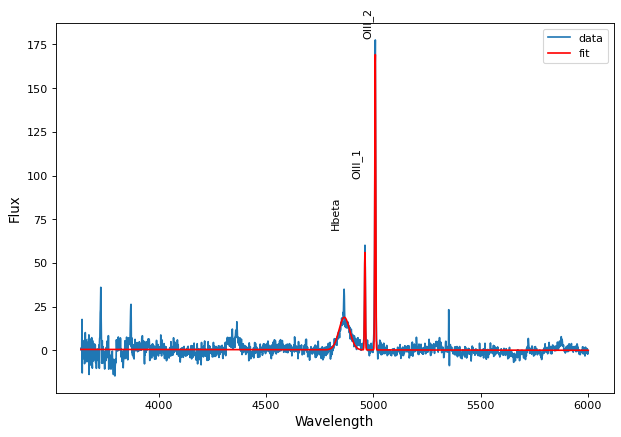
Tied Constraints
The tied constraint is often useful with Compound models.
In this example we will read a spectrum from a file called spec.txt
and fit Gaussians to the lines simultaneously while linking the flux of the OIII_1 and OIII_2 lines.
import numpy as np
from astropy.io import ascii
from astropy.utils.data import get_pkg_data_filename
from astropy.modeling import models, fitting
fname = get_pkg_data_filename('data/spec.txt', package='astropy.modeling.tests')
spec = ascii.read(fname)
wave = spec['lambda']
flux = spec['flux']

# Use the rest wavelengths of known lines as initial values for the fit.

Hbeta = 4862.721
OIII_1 = 4958.911
OIII_2 = 5008.239

# Create Gaussian1D models for each of the Hbeta and OIII lines.

h_beta = models.Gaussian1D(amplitude=34, mean=Hbeta, stddev=5)
o3_2 = models.Gaussian1D(amplitude=170, mean=OIII_2, stddev=5)
o3_1 = models.Gaussian1D(amplitude=57, mean=OIII_1, stddev=5)


# Tie the ratio of the intensity of the two OIII lines.

def tie_ampl(model):
    return model.amplitude_2 / 3.1

o3_1.amplitude.tied = tie_ampl


# Also tie the wavelength of the Hbeta line to the OIII wavelength.

def tie_wave(model):
    return model.mean_0 * OIII_1 / Hbeta

o3_1.mean.tied = tie_wave

# Create a Polynomial model to fit the continuum.

mean_flux = flux.mean()
cont = np.where(flux > mean_flux, mean_flux, flux)
linfitter = fitting.LinearLSQFitter()
poly_cont = linfitter(models.Polynomial1D(1), wave, cont)

# Create a compound model for the three lines and the continuum.

hbeta_combo = h_beta + o3_1 + o3_2 + poly_cont

# Fit all lines simultaneously -
# this will need one iteration more than the default of 100.

fitter = fitting.LevMarLSQFitter()
fitted_model = fitter(hbeta_combo, wave, flux, maxiter=111)
fitted_lines = fitted_model(wave)

from matplotlib import pyplot as plt
fig = plt.figure(figsize=(9, 6))
p = plt.plot(wave, flux, label="data")
p = plt.plot(wave, fitted_lines, 'r', label="fit")
p = plt.legend()
p = plt.xlabel("Wavelength")
p = plt.ylabel("Flux")
t = plt.text(4800, 70, 'Hbeta', rotation=90)
t = plt.text(4900, 100, 'OIII_1', rotation=90)
t = plt.text(4950, 180, 'OIII_2', rotation=90)
plt.show()