Convolution Kernels

Introduction and Concept

The convolution module provides several built-in kernels to cover the most common applications in astronomy. It is also possible to define custom kernels from arrays or combine existing kernels to match specific applications.

Every filter kernel is characterized by its response function. For time series we speak of an “impulse response function” or for images we call it “point spread function.” This response function is given for every kernel by a FittableModel, which is evaluated on a grid with discretize_model() to obtain a kernel array, which can be used for discrete convolution with the binned data.

Examples

1D Kernels

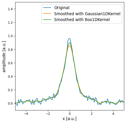
One application of filtering is to smooth noisy data. In this case we consider a noisy Lorentz curve:

>>> import numpy as np
>>> from astropy.modeling.models import Lorentz1D
>>> from astropy.convolution import convolve, Gaussian1DKernel, Box1DKernel
>>> rng = np.random.default_rng()
>>> lorentz = Lorentz1D(1, 0, 1)
>>> x = np.linspace(-5, 5, 100)
>>> data_1D = lorentz(x) + 0.1 * (rng.random(100) - 0.5)

Smoothing the noisy data with a Gaussian1DKernel with a standard deviation of 2 pixels:

>>> gauss_kernel = Gaussian1DKernel(2)
>>> smoothed_data_gauss = convolve(data_1D, gauss_kernel)

Smoothing the same data with a Box1DKernel of width 5 pixels:

>>> box_kernel = Box1DKernel(5)
>>> smoothed_data_box = convolve(data_1D, box_kernel)

The following plot illustrates the results:

(png, svg, pdf)

Beside the astropy convolution functions convolve and convolve_fft, it is also possible to use the kernels with numpy or scipy convolution by passing the array attribute. This will be faster in most cases than the astropy convolution, but will not work properly if NaN values are present in the data.

>>> smoothed = np.convolve(data_1D, box_kernel.array)

2D Kernels

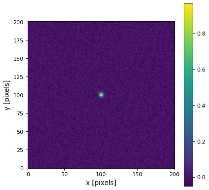
As all 2D kernels are symmetric, it is sufficient to specify the width in one direction. Therefore the use of 2D kernels is basically the same as for 1D kernels. Here we consider a small Gaussian-shaped source of amplitude 1 in the middle of the image and add 10% noise:

>>> import numpy as np
>>> from astropy.convolution import convolve, Gaussian2DKernel, Tophat2DKernel
>>> from astropy.modeling.models import Gaussian2D
>>> gauss = Gaussian2D(1, 0, 0, 3, 3)
>>> # Fake image data including noise
>>> rng = np.random.default_rng()
>>> x = np.arange(-100, 101)
>>> y = np.arange(-100, 101)
>>> x, y = np.meshgrid(x, y)
>>> data_2D = gauss(x, y) + 0.1 * (rng.random((201, 201)) - 0.5)

Smoothing the noisy data with a Gaussian2DKernel with a standard deviation of 2 pixels:

>>> gauss_kernel = Gaussian2DKernel(2)
>>> smoothed_data_gauss = convolve(data_2D, gauss_kernel)

Smoothing the noisy data with a Tophat2DKernel of width 5 pixels:

>>> tophat_kernel = Tophat2DKernel(5)
>>> smoothed_data_tophat = convolve(data_2D, tophat_kernel)

This is what the original image looks like:

(png, svg, pdf)

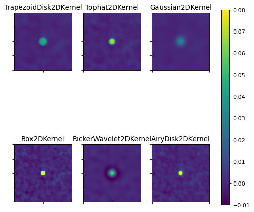
The following plot illustrates the differences between several 2D kernels applied to the simulated data. Note that it has a slightly different color scale compared to the original image.

(png, svg, pdf)

The Gaussian kernel has better smoothing properties compared to the Box and the Top Hat. The Box filter is not isotropic and can produce artifacts (the source appears rectangular). The Ricker Wavelet filter removes noise and slowly varying structures (i.e., background), but produces a negative ring around the source. The best choice for the filter strongly depends on the application.

Available Kernels

AiryDisk2DKernel(radius, **kwargs)	2D Airy disk kernel.
Box1DKernel(width, **kwargs)	1D Box filter kernel.
Box2DKernel(width, **kwargs)	2D Box filter kernel.
CustomKernel(array)	Create filter kernel from list or array.
Gaussian1DKernel(stddev, **kwargs)	1D Gaussian filter kernel.
Gaussian2DKernel(x_stddev[, y_stddev, theta])	2D Gaussian filter kernel.
RickerWavelet1DKernel(width, **kwargs)	1D Ricker wavelet filter kernel (sometimes known as a "Mexican Hat" kernel).
RickerWavelet2DKernel(width, **kwargs)	2D Ricker wavelet filter kernel (sometimes known as a "Mexican Hat" kernel).
Model1DKernel(model, **kwargs)	Create kernel from 1D model.
Model2DKernel(model, **kwargs)	Create kernel from 2D model.
Moffat2DKernel(gamma, alpha, **kwargs)	2D Moffat kernel.
Ring2DKernel(radius_in, width, **kwargs)	2D Ring filter kernel.
Tophat2DKernel(radius, **kwargs)	2D Tophat filter kernel.
Trapezoid1DKernel(width[, slope])	1D trapezoid kernel.
TrapezoidDisk2DKernel(radius[, slope])	2D trapezoid kernel.

Kernel Arithmetics

Addition and Subtraction

As convolution is a linear operation, kernels can be added or subtracted from each other. They can also be multiplied with some number.

Examples

One basic example of subtracting kernels would be the definition of a Difference of Gaussian filter:

>>> from astropy.convolution import Gaussian1DKernel
>>> gauss_1 = Gaussian1DKernel(10)
>>> gauss_2 = Gaussian1DKernel(16)
>>> DoG = gauss_2 - gauss_1

Another application is to convolve faked data with an instrument response function model. For example, if the response function can be described by the weighted sum of two Gaussians:

>>> gauss_1 = Gaussian1DKernel(10)
>>> gauss_2 = Gaussian1DKernel(16)
>>> SoG = 4 * gauss_1 + gauss_2

Most times it will be necessary to normalize the resulting kernel by calling explicitly:

>>> SoG.normalize()

Convolution

Furthermore, two kernels can be convolved with each other, which is useful when data is filtered with two different kinds of kernels or to create a new, special kernel.

Examples

To convolve two kernels with each other:

>>> from astropy.convolution import Gaussian1DKernel, convolve
>>> gauss_1 = Gaussian1DKernel(10)
>>> gauss_2 = Gaussian1DKernel(16)
>>> broad_gaussian = convolve(gauss_2,  gauss_1)  

Or in case of multistage smoothing:

>>> import numpy as np
>>> from astropy.modeling.models import Lorentz1D
>>> from astropy.convolution import convolve, Gaussian1DKernel, Box1DKernel
>>> rng = np.random.default_rng()
>>> lorentz = Lorentz1D(1, 0, 1)
>>> x = np.linspace(-5, 5, 100)
>>> data_1D = lorentz(x) + 0.1 * (rng.random(100) - 0.5)

>>> gauss = Gaussian1DKernel(3)
>>> box = Box1DKernel(5)
>>> smoothed_gauss = convolve(data_1D, gauss)
>>> smoothed_gauss_box = convolve(smoothed_gauss, box)

You would rather do the following:

>>> gauss = Gaussian1DKernel(3)
>>> box = Box1DKernel(5)
>>> smoothed_gauss_box = convolve(data_1D, convolve(box, gauss))  

Which, in most cases, will also be faster than the first method because only one convolution with the often times larger data array will be necessary.

Discretization

To obtain the kernel array for discrete convolution, the kernel’s response function is evaluated on a grid with discretize_model(). For the discretization step the following modes are available:

• Mode 'center' (default) evaluates the response function on the grid by taking the value at the center of the bin.

  >>> from astropy.convolution import Gaussian1DKernel
  >>> gauss_center = Gaussian1DKernel(3, mode='center')
  

• Mode 'linear_interp' takes the values at the corners of the bin and linearly interpolates the value at the center:

  >>> gauss_interp = Gaussian1DKernel(3, mode='linear_interp')
  

• Mode 'oversample' evaluates the response function by taking the mean on an oversampled grid. The oversample factor can be specified with the factor argument. If the oversample factor is too large, the evaluation becomes slow.

>>> gauss_oversample = Gaussian1DKernel(3, mode='oversample', factor=10)

• Mode 'integrate' integrates the function over the pixel using scipy.integrate.quad and scipy.integrate.dblquad. This mode is very slow and is only recommended when the highest accuracy is required.

>>> gauss_integrate = Gaussian1DKernel(3, mode='integrate')

Especially in the range where the kernel width is in order of only a few pixels, it can be advantageous to use the mode oversample or integrate to conserve the integral on a subpixel scale.

Normalization

The kernel models are normalized per default (i.e., \(\int_{-\infty}^{\infty} f(x) dx = 1\)). But because of the limited kernel array size, the normalization for kernels with an infinite response can differ from one. The value of this deviation is stored in the kernel’s truncation attribute.

The normalization can also differ from one, especially for small kernels, due to the discretization step. This can be partly controlled by the mode argument, when initializing the kernel. (See also discretize_model().) Setting the mode to 'oversample' allows us to conserve the normalization even on the subpixel scale.

The kernel arrays can be renormalized explicitly by calling either the normalize() method or by setting the normalize_kernel argument in the convolve() and convolve_fft() functions. The latter method leaves the kernel itself unchanged but works with an internal normalized version of the kernel.

Note that for RickerWavelet1DKernel and RickerWavelet2DKernel there is \(\int_{-\infty}^{\infty} f(x) dx = 0\). To define a proper normalization, both filters are derived from a normalized Gaussian function.