Plotting with Astroplan
astroplan currently has convenience functions for making three different types
of plots: airmass vs time, parallactic angle vs time and sky charts. This
plotting functionality in astroplan requires Matplotlib (although non-
plotting functionality will work even without Matplotlib ). The use of
additional plotting packages (like Seaborn) is not explicitly prevented,
but may or may not actually work.
All astroplan plots return a Axes object (which by
convention is assigned to the name ax in these tutorials). You can further
manipulate the returned ax object, including using it as input for more
astroplan plotting functions, or you can simply display/print the plot.
Contents
Time Dependent Plots
Although all astroplan plots are time-dependent in some way, we label those
that have a time-based axis as “time-dependent”.
astroplan currently has a few different types of “time-dependent” plots,
for example plot_airmass, plot_altitude
and plot_parallactic. These take, at minimum,
Observer, FixedTarget and Time objects
as input.
Airmass vs time plots are made the following way:
>>> from astroplan.plots import plot_airmass

>>> plot_airmass(target, observer, time)
Parallactic angle vs time plots are made the following way:
>>> from astroplan.plots import plot_airmass

>>> plot_parallactic(target, observer, time)
Below are general guidelines for working with time-dependent plots in
astroplan. Examples use airmass but apply to parallactic angle as well.
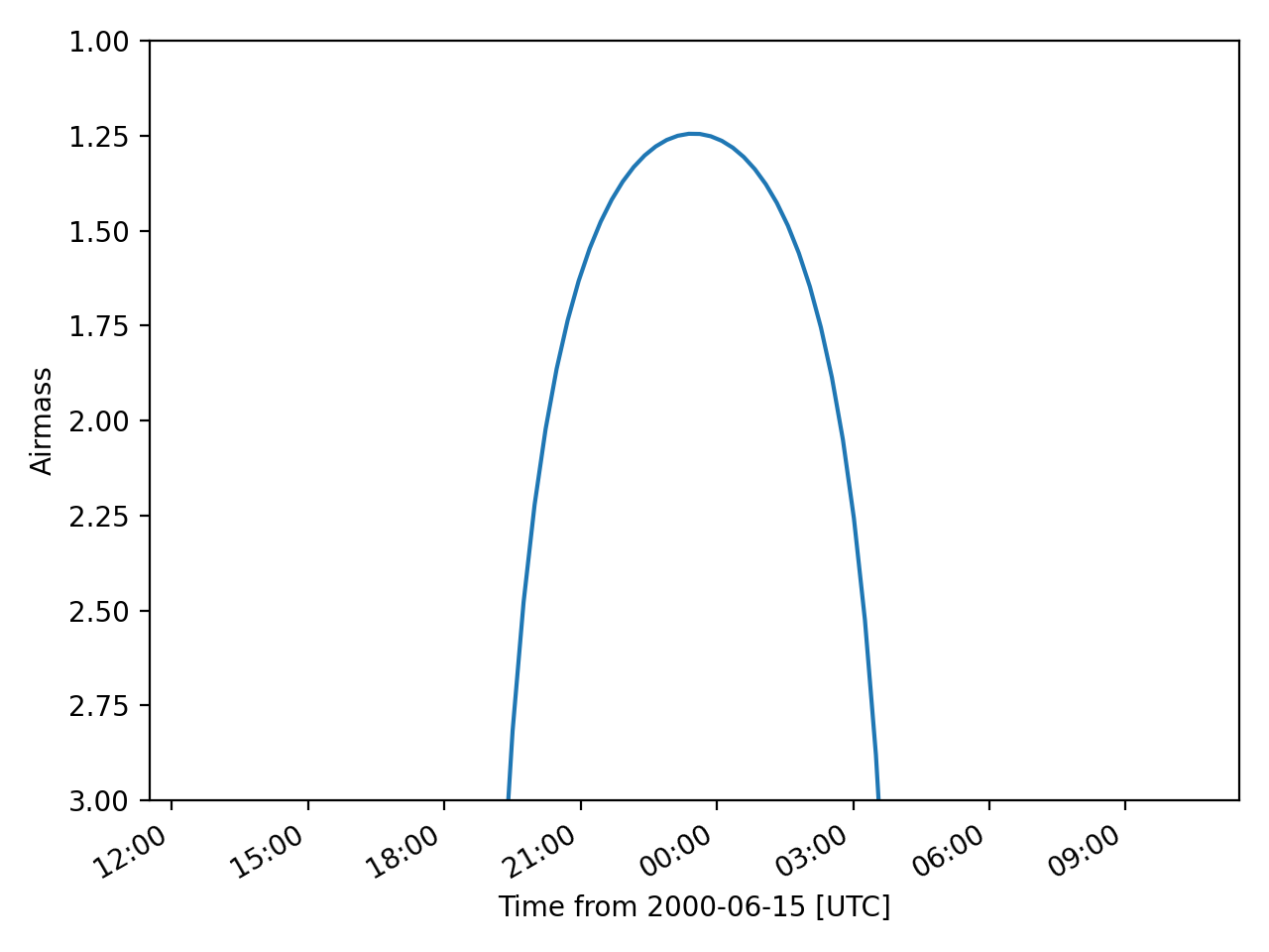
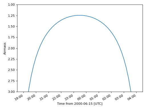
Making a quick plot
Any plot function in astroplan with a time-based axis will allow you to make
a quick plot over a 24-hour period.
After constructing Observer and FixedTarget
objects, construct a Time object with a single instance in
time and issue the plotting command.
>>> import matplotlib.pyplot as plt
>>> from astropy.time import Time
>>> from astroplan.plots import plot_airmass

>>> observe_time = Time('2000-06-15 23:30:00')

>>> plot_airmass(target, observer, observe_time)
>>> plt.show()
(Source code, png, hires.png, pdf)

As you can see, the 24-hour plot is centered on the time input. You can also
use array Time objects for these quick plots–they just
can’t contain more than one instance in time.
For example, these are acceptable time inputs:
Time(['2000-06-15 23:30:00'])

[Time('2000-06-15 23:30:00')]
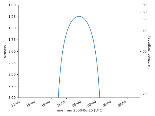
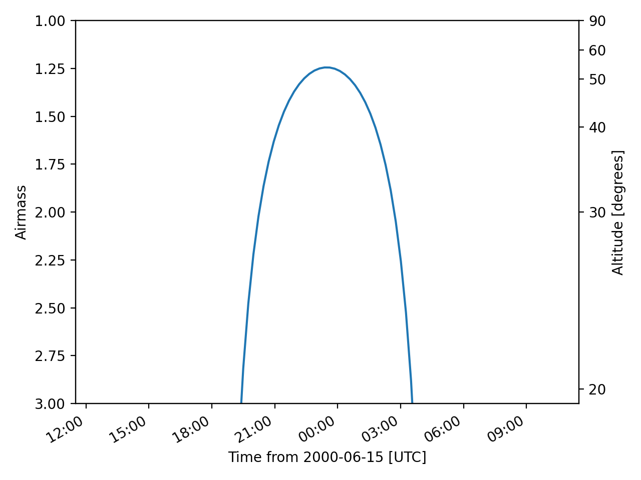
You can also add a second y-axis (on the right side) which shows the corresponding altitude of the targets:
(Source code, png, hires.png, pdf)

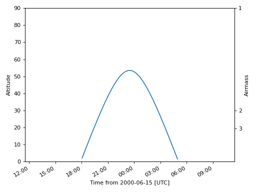
You can make altitude the primary y-axis rather than airmass by using
plot_altitude:
(Source code, png, hires.png, pdf)

Specifying a time window
If you want to see airmass plotted over a window that is not 24 hours long or
you want to control the precision of the plot, you must specify every time for
which you want to see an airmass plotted. Therefore, an array
Time object is necessary.
To quickly populate an Time object with many instances of time,
use Numpy and units. See example below.
Centering the window at some time
To center your window at some instance in time:
>>> import numpy as np
>>> import matplotlib.pyplot as plt
>>> import astropy.units as u
>>> from astropy.time import Time
>>> from astroplan.plots import plot_airmass

>>> observe_time = Time('2000-06-15 23:30:00')
>>> observe_time = observe_time + np.linspace(-5, 5, 55)*u.hour

>>> plot_airmass(target, observer, observe_time)
>>> plt.show()
(Source code, png, hires.png, pdf)

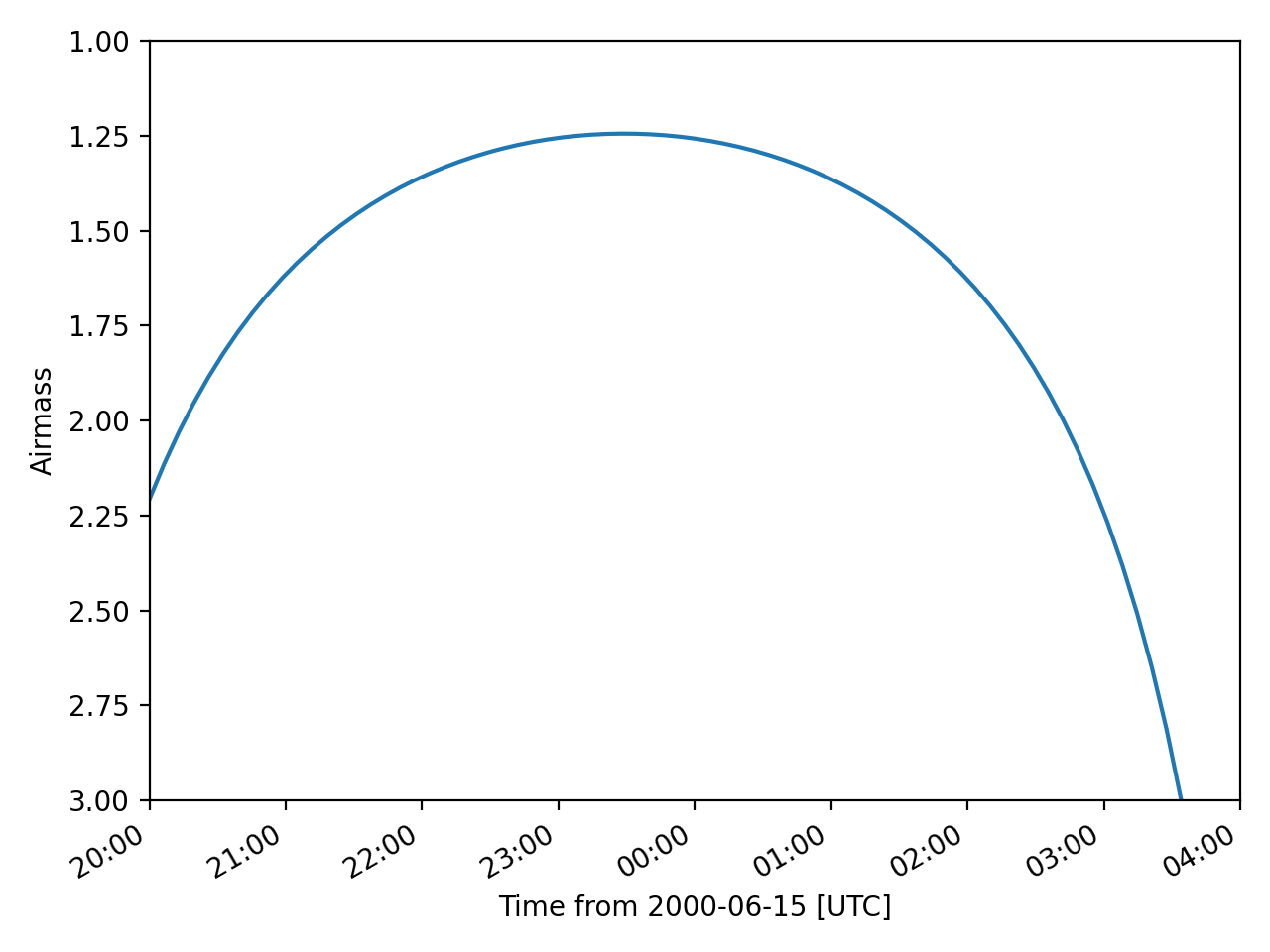
Specify start and end times
If you know the start and end times of your observation run, you can use a
TimeDelta object to create an array for time input:
>>> import numpy as np
>>> import matplotlib.pyplot as plt
>>> from astropy.time import Time
>>> from astroplan.plots import plot_airmass

>>> start_time = Time('2000-06-15 20:00:00')
>>> end_time = Time('2000-06-16 04:00:00')
>>> delta_t = end_time - start_time
>>> observe_time = start_time + delta_t*np.linspace(0, 1, 75)

>>> plot_airmass(target, observer, observe_time)
>>> plt.show()
(Source code, png, hires.png, pdf)

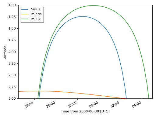
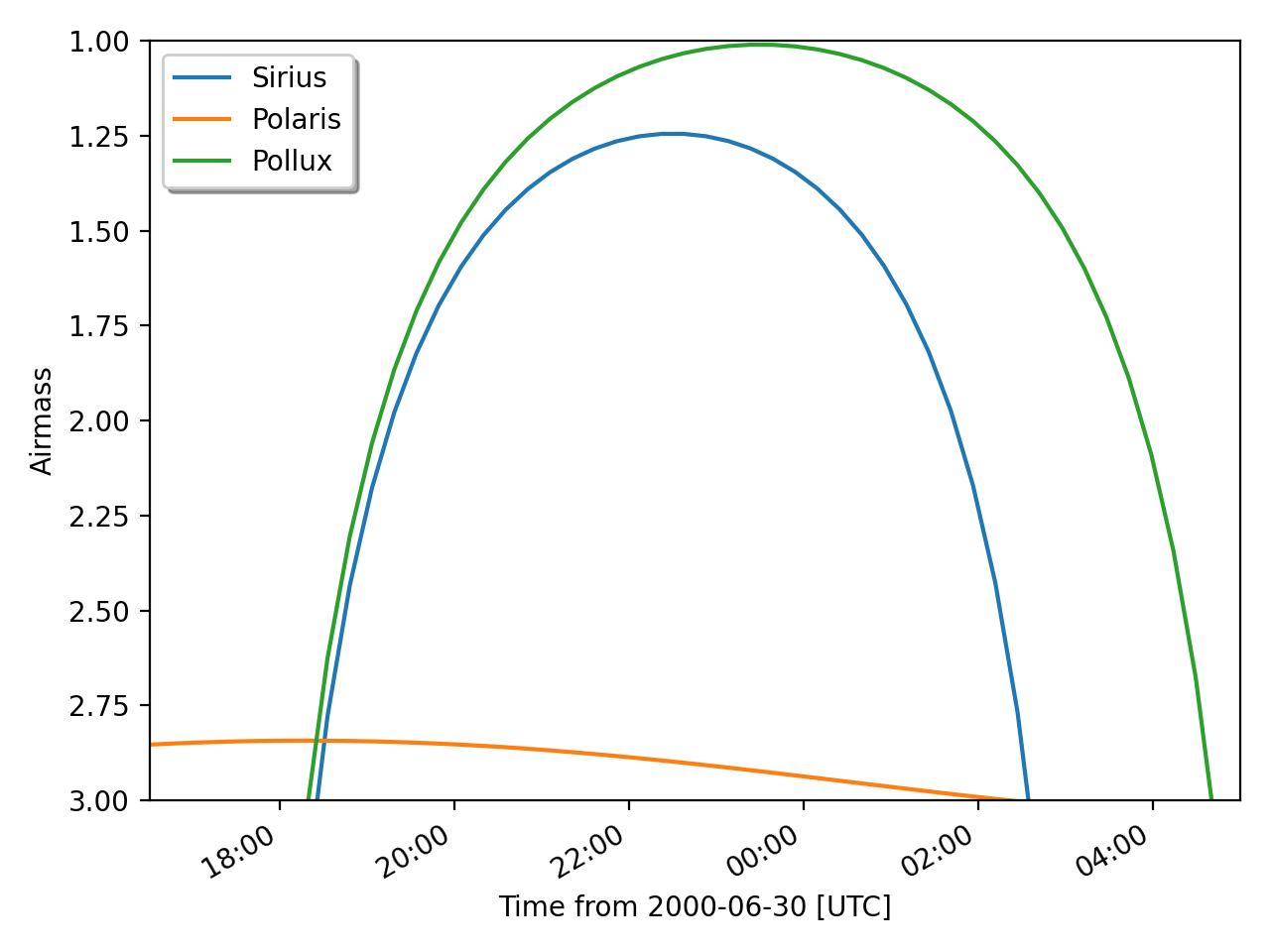
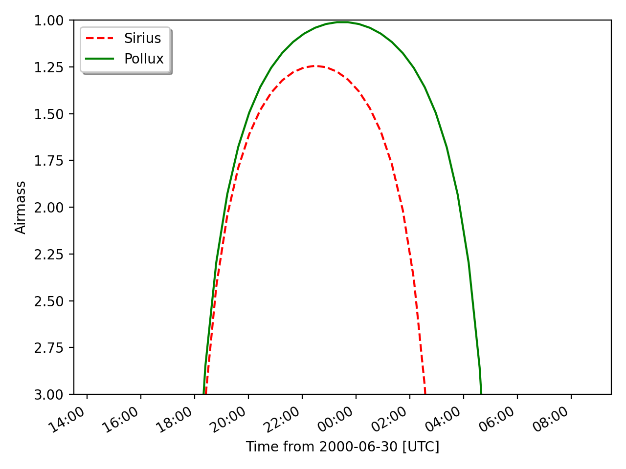
Plotting a quantity for multiple targets
If you want to plot airmass information for multiple targets, simply reissue
the plot_airmass command, using a different
FixedTarget object as input this time. Repeat until you have as
many targets on the plot as you wish:
>>> import numpy as np
>>> import matplotlib.pyplot as plt
>>> from astropy.time import Time
>>> from astroplan.plots import plot_airmass

>>> observe_time = Time('2000-06-30 23:30:00') + np.linspace(-7.0, 5.5, 50)*u.hour

>>> plot_airmass(target, observer, observe_time)
>>> plot_airmass(other_target, observer, observe_time)
>>> plot_airmass(third_target, observer, observe_time)

>>> plt.legend(shadow=True, loc=2)
>>> plt.show()
(Source code, png, hires.png, pdf)

When you’re ready to make a different plot, use ax.cla() to clear the
current Axes object.
Changing style options
The default line for time-dependent plots is solid and the default label
(should you choose to display a legend) is the name contained in the
Target object. You can change the linestyle, color,
label and other plotting properties by setting the style_kwargs option.
>>> import matplotlib.pyplot as plt
>>> from astroplan.plots import plot_airmass

>>> sirius_styles = {'linestyle': '--', 'color': 'r'}
>>> pollux_styles = {'color': 'g'}

>>> plot_airmass(target, observer, observe_time, style_kwargs=sirius_styles)
>>> plot_airmass(other_target, observer, observe_time, style_kwargs=pollux_styles)

>>> plt.legend(shadow=True, loc=2)
>>> plt.show()
(Source code, png, hires.png, pdf)

See the Matplotlib documentation for information on plotting styles in line plots.
Dark Theme Plots
By default, astroplan uses the `astropy`_ style sheet for Matplotlib to
generate plots with more pleasing settings than provided for by the matplotlib
defaults. When using astroplan at night, you may prefer to make plots with
dark backgrounds, rather than the default white background, to preserve your
night vision. To do so, you may use the astroplan dark style sheet to
produce dark-themed plots by using the style_sheet keyword argument in
any plotting function:
>>> from astroplan.plots import dark_style_sheet, plot_airmass
>>> plot_airmass(target, observatory, time, style_sheet=dark_style_sheet)
Additional Options
You can also shade the background according to the darkness of the sky (light
shading for 0 degree twilight, darker shading for -18 degree twilight) with
the brightness_shading keyword, and display additional y-axis ticks on the
right side of the axis with the altitudes in degrees using the
altitude_yaxis keyword:
>>> import matplotlib.pyplot as plt
>>> from astropy.time import Time
>>> from astroplan import FixedTarget, Observer
>>> from astroplan.plots import plot_airmass

>>> time = Time('2018-01-02 19:00')
>>> target = FixedTarget.from_name('HD 189733')
>>> apo = Observer.at_site('APO')
>>> plot_airmass(target, apo, time, brightness_shading=True, altitude_yaxis=True)
Sky Charts
Many users planning an observation run will want to see the positions of targets with respect to their local horizon, as well as the positions of familiar stars or other objects to act as guides.
plot_sky allows you to plot the positions of targets at a
single instance or over some window of time. You make this plot the
following way:
>>> from astroplan.plots import plot_sky

>>> plot_sky(target, observer, time)
Note
plot_sky currently produces polar plots in
altitude/azimuth coordinates only. Plots are centered on the observer’s
zenith.
See also
Making a plot for one instance in time
After constructing your Observer and FixedTarget
objects, construct a time input using an array of length 1.
That is, either an Time object with an array containing one
time value (e.g., Time(['2000-1-1'])) or an array containing one scalar
Time object (e.g., [Time('2000-1-1')]).
Let’s say that you created FixedTarget objects for Polaris,
Altair, Vega and Deneb. To plot a map of the sky:
>>> import matplotlib.pyplot as plt
>>> from astropy.time import Time
>>> from astroplan.plots import plot_sky

>>> observe_time = Time(['2000-03-15 15:30:00'])

>>> polaris_style = {color': 'k'}
>>> vega_style = {'color': 'g'}
>>> deneb_style = {'color': 'r'}

>>> plot_sky(polaris, observer, observe_time, style_kwargs=polaris_style)
>>> plot_sky(altair, observer, observe_time)
>>> plot_sky(vega, observer, observe_time, style_kwargs=vega_style)
>>> plot_sky(deneb, observer, observe_time, style_kwargs=deneb_style)

>>> plt.legend(loc='center left', bbox_to_anchor=(1.25, 0.5))
>>> plt.show()
Note
Since plot_sky uses scatter
(which gives the same color to different plots made on the same set of
axes), you have to specify the color for each target via a style
dictionary if you don’t want all targets to have the same color.
Showing movement over time
If you want to see how your targets move over time, you need to explicitly specify every instance in time.
Say I want to know how Altair moves in the sky over a 9-hour period:
>>> import numpy as np
>>> import matplotlib.pyplot as plt
>>> import astropy.units as u
>>> from astroplan.plots import plot_sky

>>> observe_time = Time('2000-03-15 17:00:00')
>>> observe_time = observe_time + np.linspace(-4, 5, 10)*u.hour

>>> plot_sky(altair, observer, observe_time)

>>> plt.legend(loc='center left', bbox_to_anchor=(1.25, 0.5))
>>> plt.show()
For more examples on how to populate time objects, see Time
documentation, or Specifying a time window.
Note
Note that in the case of an object being under the horizon (or having
negative altitude) at any of the times in your time input,
plot_sky will warn you. Your object(s) will not show
up on the plot for those particular times, but any positions above the
horizon will still be plotted as normal.
Customizing your sky plot
astroplan plots use Matplotlib defaults, so you can customize your plots in
much the same way you tweak any Matplotlib plot.
Setting style options
The default marker for plot_sky is a circle and the
default label (should you choose to display a legend) is the name contained
in the Target object. You can change the marker, color,
label and other plotting properties by setting the style_kwargs option,
in the same way shown for the time-dependent plots.
One situation in which this is particularly useful is the plotting of guide positions, such as a few familiar stars or any body used in calibrating your telescope. You can also use this feature to set apart different types of targets (e.g., high-priority, candidates for observing run, etc.).
See the Matplotlib documentation for information on plotting styles in scatter plots.
Changing coordinate defaults
As seen in the above examples, the default position of North is at the top of the plot, and South at the bottom, with azimuth increasing counter-clockwise (CCW), putting East to the left, and West to the right.
You can’t change the position of North or South (either in the actual plotting of the data, or the labels), but you can “flip” East/West by changing the direction in which azimuth increases via the north_to_east_ccw option:
>>> import matplotlib.pyplot as plt
>>> from astroplan.plots import plot_sky

>>> guide_style = {'marker': '*'}

>>> plot_sky(polaris, observer, observe_time, snorth_to_east_ccw=False, style_kwargs=guide_style)
>>> plot_sky(altair, observer, observe_time, north_to_east_ccw=False)

>>> plt.legend(loc='center left', bbox_to_anchor=(1.25, 0.5))
>>> plt.show()
Some observatories may need to offset or rotate the azimuth labels due to their particular telescope setup.
To do this, set az_label_offset equal to the number of degrees by which you wish to rotate the labels. By default, az_label_offset is set to 0 degrees. A positive offset is in the same direction as azimuth increase (see the north_to_east_ccw option):
>>> import matplotlib.pyplot as plt
>>> from astroplan.plots import plot_sky

>>> guide_style = {'marker': '*'}

>>> plot_sky(polaris, observer, observe_time, style_kwargs=guide_style, az_label_offset=180.0*u.deg)
>>> plot_sky(altair, observer, observe_time, az_label_offset=180.0*u.deg)

>>> plt.legend(loc='center left', bbox_to_anchor=(1.25, 0.5))
>>> plt.show()
Note
The az_label_offset option does not rotate the actual positions on the
plot, but simply the theta grid labels (which are drawn regardless of
gridline presence). Since labels are drawn with every call to
plot_sky, we recommend you use the same
az_label_offset argument for every target on the same plot.
It is not advised that most users change this option, as it may appear that your alt/az data does not coincide with the definition of altazimuth (local horizon) coordinate system.
You can turn off the grid lines by setting the grid option to False:
>>> import matplotlib.pyplot as plt
>>> from astroplan.plots import plot_sky

>>> guide_style = {'marker': '*'}

>>> plot_sky(polaris, observer, observe_time, style_kwargs=guide_style, grid=False)
>>> plot_sky(altair, observer, observe_time, grid=False)

>>> plt.legend(loc='center left', bbox_to_anchor=(1.25, 0.5))
>>> plt.show()
Note
Since grids are redrawn with every call to plot_sky,
you must set grid=False for every target in the same plot.
Other tweaks
You can easily change other plot attributes by acting on the returned
matplotlib.axes.Axes object or via matplotlib.pyplot calls (e.g.,
plt.figure, plt.rc, etc.).
For instance, you can increase the size of your plot and its font:
>>> # Set the figure size/font before you issue the plotting command.
>>> plt.figure(figsize=(8,6))
>>> plt.rc('font', size=14)

>>> plot_sky(polaris, observer, observe_time)
>>> plot_sky(altair, observer, observe_time)

>>> plt.legend(loc='center left', bbox_to_anchor=(1.25, 0.5))
>>> plt.show()

>>> # Change font size back to default once done plotting.
>>> plt.rc('font', size=12)
Miscellaneous
The easiest way to reuse the Axes object that is the base of
your plots is to just let astroplan’s plotting functions take care of it in
the background. You do, however, have the option of explicitly passing in a
named axis, assuming that you have created the appropriate type for the
particular plot you want.
We can explicitly give a name to the Axes object returned
by plot_sky when plotting Polaris and reuse it to plot
Altair:
>>> my_ax = plot_sky(polaris, observer, observe_time, style_kwargs=guide_style)
>>> plot_sky(altair, observer, observe_time, my_ax)
We can also create a Axes object entirely outside of
plot_sky, then pass it in:
>>> my_ax = plt.gca(projection='polar')
>>> plot_sky(polaris, observer, observe_time, my_ax)
Passing in named matplotlib.axes.Axes objects comes in handy when you want to
make multiple plots:
>>> from astroplan.plots import plot_sky
>>> import matplotlib.pyplot as plt

>>> my_ax = plot_sky(polaris, observer, observe_time, style_kwargs=polaris_style)
>>> plot_sky(altair, observer, observe_time, my_ax, style_kwargs=altair_style)
>>> plt.legend(loc='center left', bbox_to_anchor=(1.3, 0.5))

>>> # Note that this plt.show (or another action, such as saving a figure) is critical in maintaining two separate plots.
>>> plt.show()

>>> other_ax = plot_sky(vega, observer, observe_time, style_kwargs=vega_style)
>>> plot_sky(deneb, observer, observe_time, other_ax, style_kwargs=deneb_style)
>>> plt.legend(loc='center left', bbox_to_anchor=(1.25, 0.5))
>>> plt.show()
Finder Chart/Image
astroplan includes a function for generating quick finder images from
Python, plot_finder_image, by querying for images from
sky surveys centered on a FixedTarget. This function depends on
astroquery (in addition to Matplotlib). In this example, we’ll quickly
make a finder image centered on The Crab Nebula (M1):
>>> from astroplan.plots import plot_finder_image
>>> from astroplan import FixedTarget
>>> import matplotlib.pyplot as plt

>>> messier1 = FixedTarget.from_name("M1")
>>> ax, hdu = plot_finder_image(messier1)
>>> plt.show()