Inpainting missing data#
Missing data in an image can be an issue, especially when one wants to perform Fourier analysis. This tutorial explains how to fill-up missing pixels with values which looks “realistic” and introduce as little perturbation as possible for subsequent analysis. The user should keep the mask nearby and only consider the values of actual pixels and never the one inpainted.
This tutorial will use fully synthetic data to allow comparison between actual (syntetic) data with inpainted values.
The first part of the tutorial is about the generation of a challenging 2D diffraction image with realistic noise and to describe the metric used, then comes the actual tutorial on how to use the inpainting. Finally a benchmark is used based on the metric determined.
Creation of the image#
A realistic challenging image should contain:
Bragg peak rings. We chose LaB6 as guinea-pig, with very sharp peaks, at the limit of the resolution of the detector
Some amorphous content
strong polarization effect
Poissonian noise
One image will be generated but then multiple ones with different noise to discriminate the effect of the noise from other effects.
[1]:
%matplotlib inline
# Used for documentation to inline plots into notebook
# %matplotlib widget
# uncomment the later for better UI
from matplotlib.pyplot import subplots
import numpy
[2]:
import pyFAI
print("Using pyFAI version: ", pyFAI.version)
from pyFAI.gui import jupyter
import pyFAI.test.utilstest
from pyFAI.calibrant import get_calibrant
import time
start_time = time.perf_counter()
Using pyFAI version: 2025.3.0
[3]:
detector = pyFAI.detector_factory("Pilatus2MCdTe")
mask = detector.mask.copy()
nomask = numpy.zeros_like(mask)
detector.mask=nomask
ai = pyFAI.load({"detector":detector})
ai.setFit2D(200, 200, 200)
ai.wavelength = 3e-11
print(ai)
Detector Pilatus CdTe 2M         PixelSize= 172µm, 172µm         BottomRight (3)
Wavelength= 3.000000e-11 m
SampleDetDist= 2.000000e-01 m   PONI= 3.440000e-02, 3.440000e-02 m      rot1=0.000000  rot2=0.000000  rot3=0.000000 rad
DirectBeamDist= 200.000 mm      Center: x=200.000, y=200.000 pix        Tilt= 0.000° tiltPlanRotation= 0.000° 𝛌= 0.300Å
[4]:
LaB6 = get_calibrant("LaB6")
LaB6.wavelength = ai.wavelength
print(LaB6)
r = ai.array_from_unit(unit="q_nm^-1")
decay_b = numpy.exp(-(r-50)**2/2000)
bragg = LaB6.fake_calibration_image(ai, Imax=1e4, W=1e-6) * ai.polarization(factor=1.0) * decay_b
decay_a = numpy.exp(-r/100)
amorphous = 1000*ai.polarization(factor=1.0)*ai.solidAngleArray() * decay_a
img_nomask = bragg + amorphous
#Not the same noise function for all images two images
img_nomask = numpy.random.poisson(img_nomask)
img_nomask2 = numpy.random.poisson(img_nomask)
img = numpy.random.poisson(img_nomask)
img[numpy.where(mask)] = -1
fig,ax = subplots(1,2, figsize=(10,5))
jupyter.display(img=img, label="With mask", ax=ax[0])
jupyter.display(img=img_nomask, label="Without mask", ax=ax[1])
LaB6 Calibrant with 640 reflections at wavelength 3e-11
[4]:
<Axes: title={'center': 'Without mask'}>
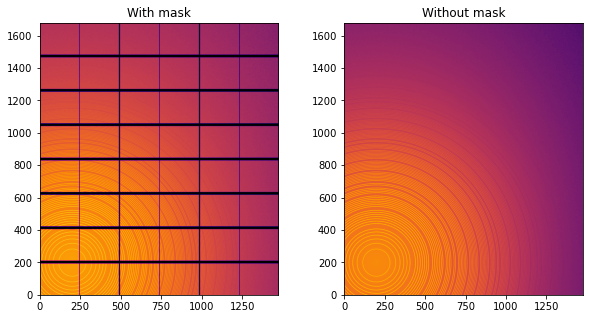
Note the aliassing effect on the displayed images.
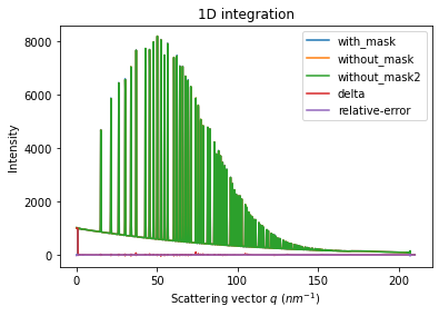
We will measure now the effect after 1D intergeration. We do not correct for polarization on purpose to highlight the defect one wishes to whipe out. We use a R-factor to describe the quality of the 1D-integrated signal.
[5]:
kwargs = {"npt":2000, "unit":"q_nm^-1", "method":("full", "histogram", "cython"), "radial_range":(0,210)}
wo = ai.integrate1d(img_nomask, **kwargs)
wo2 = ai.integrate1d(img_nomask2, **kwargs)
wm = ai.integrate1d(img, mask=mask, **kwargs)
ax = jupyter.plot1d(wm , label="with_mask")
ax.plot(*wo, label="without_mask")
ax.plot(*wo2, label="without_mask2")
ax.plot(wo.radial, wo.intensity-wm.intensity, label="delta")
ax.plot(wo.radial, wo.intensity-wo2.intensity, label="relative-error")
ax.legend()
print("Between masked and non masked image R= %s"%pyFAI.utils.mathutil.rwp(wm,wo))
print("Between two different non-masked images R'= %s"%pyFAI.utils.mathutil.rwp(wo2,wo))
Between masked and non masked image R= 5.694397862100573
Between two different non-masked images R'= 0.427194624678683
[6]:
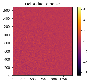
# Effect of the noise on the delta image
fig, ax = subplots()
jupyter.display(img=img_nomask-img_nomask2, label="Delta due to noise", ax=ax)
ax.figure.colorbar(ax.images[0])
[6]:
<matplotlib.colorbar.Colorbar at 0x7f0a34f7bf10>
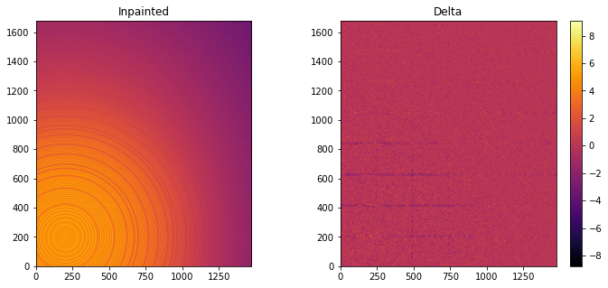
Inpainting#
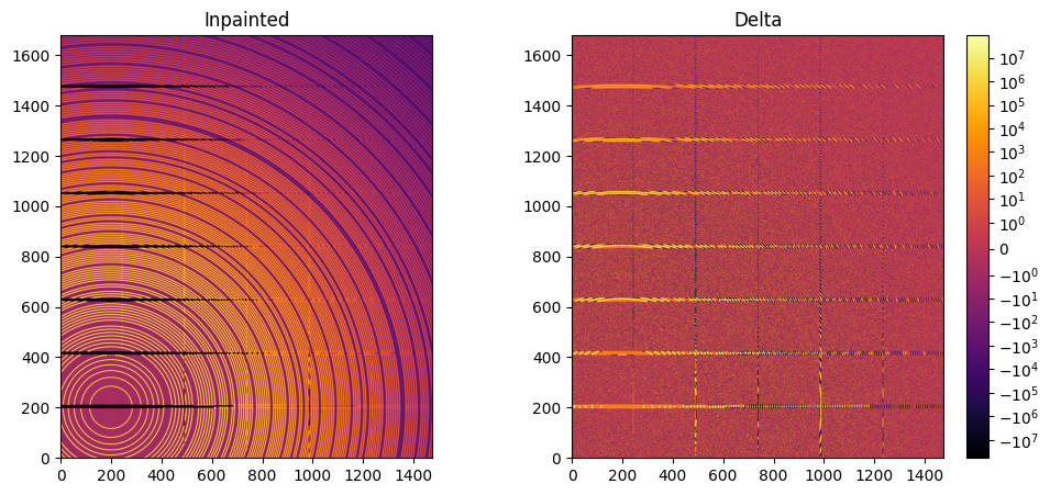
This part describes how to paint the missing pixels for having a “natural-looking image”. The delta image contains the difference with the original image
[7]:
#Inpainting:
inpainted = ai.inpainting(img, mask=mask, poissonian=True)
fig, ax = subplots(1, 2, figsize=(12,5))
jupyter.display(img=inpainted, label="Inpainted", ax=ax[0])
jupyter.display(img=img_nomask-inpainted, label="Delta", ax=ax[1])
ax[1].figure.colorbar(ax[1].images[0])
[7]:
<matplotlib.colorbar.Colorbar at 0x7f09d840a010>
[8]:
# Comparison of the inpained image with the original one:
wm = ai.integrate1d(inpainted, **kwargs)
wo = ai.integrate1d(img_nomask, **kwargs)
ax = jupyter.plot1d(wm , label="inpainted")
ax.plot(*wo, label="without_mask")
ax.plot(wo.radial, wo.intensity-wm.intensity, label="delta")
ax.legend()
print("R= %s"%pyFAI.utils.mathutil.rwp(wm,wo))
R= 27.02450730475388
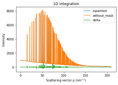
One can see by zooming in that the main effect on inpainting is a broadening of the signal in the inpainted region. This could (partially) be adressed by increasing the number of radial bins used in the inpainting.
Benchmarking and optimization of the parameters#
The parameter set depends on the detector, the experiment geometry and the type of signal on the detector. Finer detail require finer slicing.
[9]:
#Basic benchmarking of execution time for default options:
%timeit inpainted = ai.inpainting(img, mask=mask)
1.94 s ± 111 ms per loop (mean ± std. dev. of 7 runs, 1 loop each)
[10]:
wo = ai.integrate1d(img_nomask, **kwargs)
for m in (("no", "histogram", "cython"), ("bbox", "histogram","cython")):
    for k in (512, 1024, 2048, 4096):
        ai.reset()
        for i in (0, 1, 2, 4, 8):
            inpainted = ai.inpainting(img, mask=mask, poissonian=True, method=m, npt_rad=k, grow_mask=i)
            wm = ai.integrate1d(inpainted, **kwargs)
            print(f"method: {m} npt_rad={k} grow={i}; R= {pyFAI.utils.mathutil.rwp(wm,wo):.3f}")
method: ('no', 'histogram', 'cython') npt_rad=512 grow=0; R= 39.687
method: ('no', 'histogram', 'cython') npt_rad=512 grow=1; R= 39.687
method: ('no', 'histogram', 'cython') npt_rad=512 grow=2; R= 39.687
method: ('no', 'histogram', 'cython') npt_rad=512 grow=4; R= 39.687
method: ('no', 'histogram', 'cython') npt_rad=512 grow=8; R= 39.687
method: ('no', 'histogram', 'cython') npt_rad=1024 grow=0; R= 22.210
method: ('no', 'histogram', 'cython') npt_rad=1024 grow=1; R= 22.210
method: ('no', 'histogram', 'cython') npt_rad=1024 grow=2; R= 22.210
method: ('no', 'histogram', 'cython') npt_rad=1024 grow=4; R= 22.210
method: ('no', 'histogram', 'cython') npt_rad=1024 grow=8; R= 22.210
method: ('no', 'histogram', 'cython') npt_rad=2048 grow=0; R= 8.383
method: ('no', 'histogram', 'cython') npt_rad=2048 grow=1; R= 8.383
method: ('no', 'histogram', 'cython') npt_rad=2048 grow=2; R= 8.383
method: ('no', 'histogram', 'cython') npt_rad=2048 grow=4; R= 8.383
method: ('no', 'histogram', 'cython') npt_rad=2048 grow=8; R= 8.383
method: ('no', 'histogram', 'cython') npt_rad=4096 grow=0; R= 8.248
method: ('no', 'histogram', 'cython') npt_rad=4096 grow=1; R= 8.248
method: ('no', 'histogram', 'cython') npt_rad=4096 grow=2; R= 8.248
method: ('no', 'histogram', 'cython') npt_rad=4096 grow=4; R= 8.248
method: ('no', 'histogram', 'cython') npt_rad=4096 grow=8; R= 8.248
method: ('bbox', 'histogram', 'cython') npt_rad=512 grow=0; R= 41.804
method: ('bbox', 'histogram', 'cython') npt_rad=512 grow=1; R= 41.804
method: ('bbox', 'histogram', 'cython') npt_rad=512 grow=2; R= 41.802
method: ('bbox', 'histogram', 'cython') npt_rad=512 grow=4; R= 41.802
method: ('bbox', 'histogram', 'cython') npt_rad=512 grow=8; R= 41.803
method: ('bbox', 'histogram', 'cython') npt_rad=1024 grow=0; R= 28.345
method: ('bbox', 'histogram', 'cython') npt_rad=1024 grow=1; R= 28.343
method: ('bbox', 'histogram', 'cython') npt_rad=1024 grow=2; R= 28.345
method: ('bbox', 'histogram', 'cython') npt_rad=1024 grow=4; R= 28.345
method: ('bbox', 'histogram', 'cython') npt_rad=1024 grow=8; R= 28.344
method: ('bbox', 'histogram', 'cython') npt_rad=2048 grow=0; R= 12.804
method: ('bbox', 'histogram', 'cython') npt_rad=2048 grow=1; R= 12.809
method: ('bbox', 'histogram', 'cython') npt_rad=2048 grow=2; R= 12.804
method: ('bbox', 'histogram', 'cython') npt_rad=2048 grow=4; R= 12.806
method: ('bbox', 'histogram', 'cython') npt_rad=2048 grow=8; R= 12.807
method: ('bbox', 'histogram', 'cython') npt_rad=4096 grow=0; R= 8.266
method: ('bbox', 'histogram', 'cython') npt_rad=4096 grow=1; R= 8.260
method: ('bbox', 'histogram', 'cython') npt_rad=4096 grow=2; R= 8.269
method: ('bbox', 'histogram', 'cython') npt_rad=4096 grow=4; R= 8.267
method: ('bbox', 'histogram', 'cython') npt_rad=4096 grow=8; R= 8.264
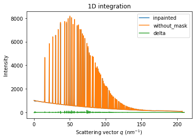
[11]:
#Inpainting, best solution found:
ai.reset()
%time inpainted = ai.inpainting(img, mask=mask, poissonian=True, method=("full", "csr", "cython"), npt_rad=4096, grow_mask=1)
fig, ax = subplots(1, 2, figsize=(12, 5))
jupyter.display(img=inpainted, label="Inpainted", ax=ax[0])
jupyter.display(img=img_nomask-inpainted, label="Delta", ax=ax[1])
ax[1].figure.colorbar(ax[1].images[0])
pass
CPU times: user 4.18 s, sys: 246 ms, total: 4.43 s
Wall time: 2.84 s
[12]:
# Comparison of the inpained image with the original one:
wm = ai.integrate1d(inpainted, **kwargs)
wo = ai.integrate1d(img_nomask, **kwargs)
ax = jupyter.plot1d(wm , label="inpainted")
ax.plot(*wo, label="without_mask")
ax.plot(wo.radial, wo.intensity-wm.intensity, label="delta")
ax.legend()
print("R= %s"%pyFAI.utils.mathutil.rwp(wm,wo))
R= 8.210758096621895
Conclusion#
Inpainting is one of the only solution to fill up the gaps in detector when Fourier analysis is needed. This tutorial explains basically how this is possible using the pyFAI library and how to optimize the parameter set for inpainting. The result may greatly vary with detector position and tilt and the kind of signal (amorphous or more spotty).
[13]:
print(f"Execution time: {time.perf_counter()-start_time:.3f} s")
Execution time: 79.292 s