Fitting wavelength with multiple sample-detector distances#
Wavelength and detector distance are correlated parameters when fitting the geometry using a single detector position. One should fix either one, or the other. The simultaneous fitting of several images taken at various detector distances has proven to alleviate this limitation (https://doi.org/10.1107/S1600577519013328).
This tutorial explains how to perform a multi-position geometry refinement, this within pyFAI using a notebook.
The dataset was recorded at the DanMAX beamline at MaxIV (Lund, Sweden) and made available by Mads Ry Jørgensen. It represents LaB6 reference material collected at 20keV at with a Pilatus detector at various distances from the sample.
Loading data#
All the data are stored into a single HDF5 file following the Nexus convention. This file has been reprocessed and differs from what is acquired at the DanMAX beamline.
[1]:
%matplotlib inline
#For documentation purpose, `inline` is used to enforce the storage of images into the notebook
# %matplotlib widget
import numpy
from matplotlib.pyplot import subplots
from pyFAI.goniometer import GeometryTransformation, ExtendedTransformation, SingleGeometry,\
                             GoniometerRefinement, Goniometer
from pyFAI.calibrant import get_calibrant
import h5py
import pyFAI
from pyFAI.gui import jupyter
import time
start_time = time.perf_counter()
import logging
logging.basicConfig(level=logging.WARNING)
print(f"Running pyFAI version {pyFAI.version}")
Running pyFAI version 2025.3.0
[2]:
#Download data from internet

from silx.resources import ExternalResources

#Comment out and configure the proxy if you are behind a firewall
#os.environ["http_proxy"] = "http://proxy.company.com:3128"

downloader = ExternalResources("pyFAI", "http://www.silx.org/pub/pyFAI/gonio/", "PYFAI_DATA")
data_file = downloader.getfile("LaB6_20keV.h5")

print("file downloaded:", data_file)
file downloaded: /tmp/pyFAI_testdata_jerome/LaB6_20keV.h5
[3]:
h5 = h5py.File(data_file)
images = h5["entry_0000/DanMAX/Pilatus/data"][()]
distances = h5["entry_0000/DanMAX/sdd/value"][()]
energy = h5["entry_0000/DanMAX/monochromator/energy"][()]
print("Distances: ", distances)
print("Energy:", energy)
LaB6 = get_calibrant("LaB6")
wavelength_guess = pyFAI.units.hc/energy*1e-10
print("Wavelength:", wavelength_guess)
LaB6.wavelength = wavelength_guess
Distances:  [174. 274. 374. 474. 574. 674.]
Energy: 20
Wavelength: 6.199209921660013e-11
[4]:
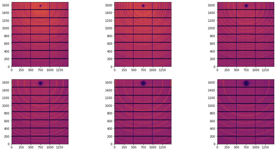
fig, ax = subplots(2,3, figsize=(18,9))
for a,i in zip(ax.ravel(), images):
    jupyter.display(i, ax=a)
[5]:
detector = pyFAI.detector_factory("Pilatus2MCdTe")
detector.mask = numpy.min(images, axis=0)<0
This dataset is composed of 6 images collected between 150 and 650 mm with a Pilatus 2M CdTe detector. Debye-Scherrer rings are very nicely visible and a fully automated calibration will be performed.
Automatic calibration#
Since those images are pretty nice, one can read the beam-center position at (x=749, y=1573, ). The tilt and other distortion will be neglected in this first stage. We will now perform the automatic ring extraction
[6]:
geometries = {}
for dist, img  in zip(distances, images):
    ai = pyFAI.load({"detector":detector, "wavelength":wavelength_guess})
    ai.setFit2D(dist, 749, 1573)
    geo = SingleGeometry(dist, img, metadata=dist, calibrant=LaB6, detector=detector, geometry=ai)
    geometries[dist] = geo
[7]:
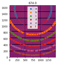
# Process the last image, the one with fewer rings:

# First extract some control points:
geo.control_points  = geo.extract_cp()
# Visualization
ax = jupyter.display(sg=geo)
[8]:
print("Optimization of the geometry ... residual error is:", geo.geometry_refinement.refine2())
print(geo.geometry_refinement)
Optimization of the geometry ... residual error is: 5.302987895783863e-09
Detector Pilatus CdTe 2M         PixelSize= 172µm, 172µm         BottomRight (3)
Wavelength= 6.199210e-11 m
SampleDetDist= 6.744392e-01 m   PONI= 2.709089e-01, 1.307619e-01 m      rot1=0.002734  rot2=0.000660  rot3=0.000000 rad
DirectBeamDist= 674.442 mm      Center: x=749.522, y=1577.640 pix       Tilt= 0.161° tiltPlanRotation= 166.429° 𝛌= 0.620Å
[9]:
# Extraction of the control points for all geometries:
fig, ax = subplots(2,3, figsize=(15, 10))
for a, lbl in zip(ax.ravel(), geometries):
    geo = geometries[lbl]
    geo.control_points  = geo.extract_cp()
#     print(geo.control_points)
    print(f"Optimization of the geometry {lbl}, residual error is: {geo.geometry_refinement.refine2()}")
    jupyter.display(sg=geo, ax=a)
a.get_legend().remove()
Optimization of the geometry 174.0, residual error is: 5.1066031562615306e-08
Optimization of the geometry 274.0, residual error is: 3.077809187622281e-08
Optimization of the geometry 374.0, residual error is: 1.6168403767781824e-08
Optimization of the geometry 474.0, residual error is: 1.0300296978343998e-08
Optimization of the geometry 574.0, residual error is: 8.360427453945028e-09
Optimization of the geometry 674.0, residual error is: 3.997742265978744e-09
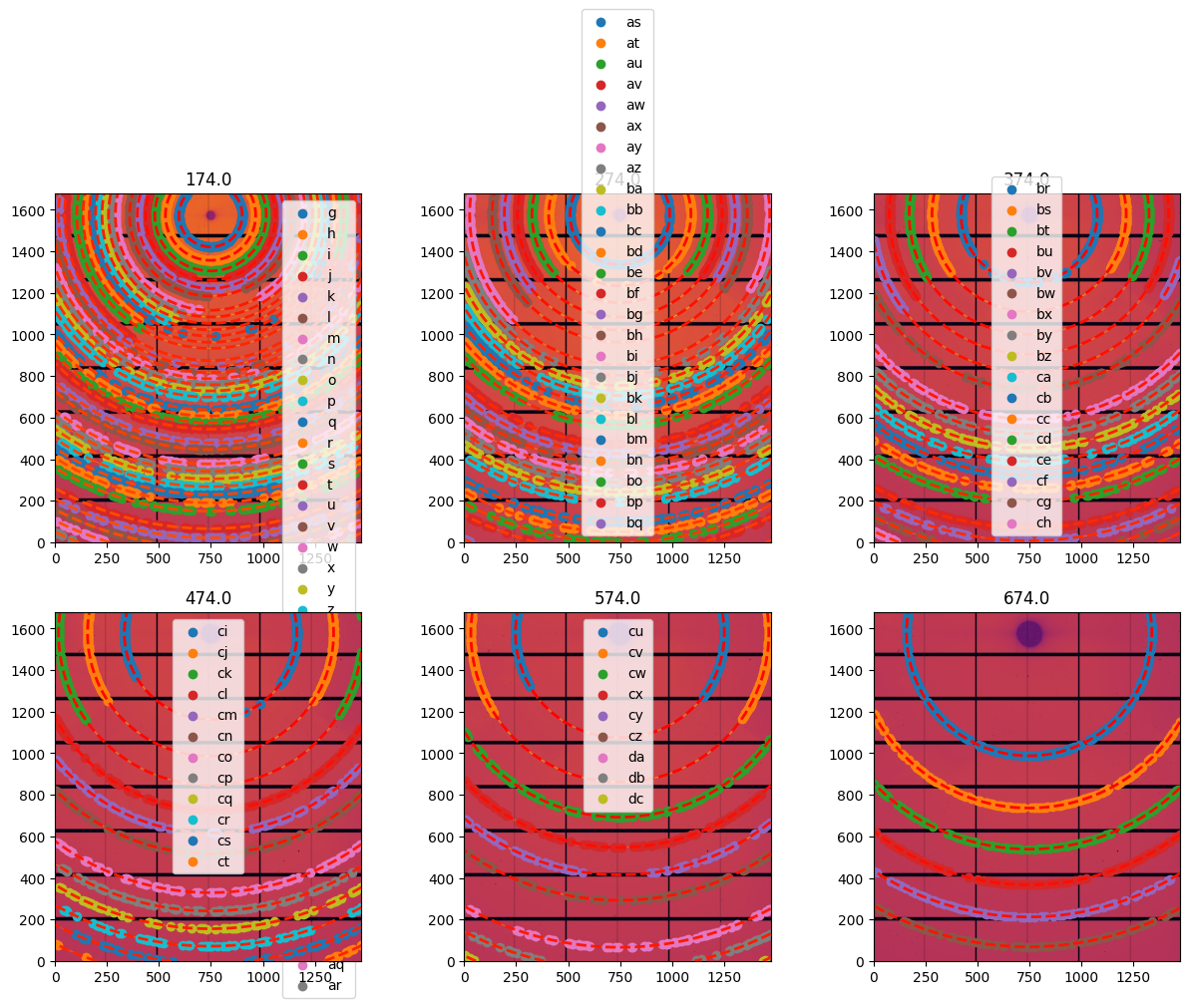
At this stage, we have 6 images and between 38 and 6 rings per image which is enough to start calibrating them all-together.
Sample stage setup#
We will optimize the energy in addition to all other parameters except the rotation along the beam (rot3).
dist0represents the offset of the sample-detector stage. The associatedscale0is expected to be 1e-3 to convert milimeters in meters.poni1represents the vertical position of the center and the associatedscale1is expected to be null.poni2represents the horizontal position of the center and the associatedscale2is expected to be null.All other rotation are expected to be null as well.
[10]:
goniotrans = ExtendedTransformation(param_names = ["dist0", "scale0",
                                                   "poni1", "scale1",
                                                   "poni2", "scale2",
                                                   "rot1", "rot2",
                                                   "energy"],
                                    dist_expr="dist0  + pos*scale0",
                                    poni1_expr="poni1 + pos*scale1",
                                    poni2_expr="poni2 + pos*scale2",
                                    rot1_expr="rot1",
                                    rot2_expr="rot2",
                                    rot3_expr="0",
                                    wavelength_expr="hc/energy*1e-10")
[11]:
# Starting parameters ...

param = {"dist0":   0.0,
         "poni1":  geo.geometry_refinement.poni1,
         "poni2":  geo.geometry_refinement.poni2,
         "rot1":   0.0,
         "rot2":   0.0,
         "scale0": 0.001,
         "scale1": 0.0,
         "scale2": 0.0,
         "energy": energy,
        }
[12]:
#Defines the bounds for some variables
bounds = {"dist0":  ( -0.1, 0.1),
          "poni1":  ( 0.0, 0.4),
          "poni2":  ( 0.0, 0.3),
          "rot1":   (-1.0, 1.0),
          "rot2":   (-1.0, 1.0),
          "scale0": (-1.1, 1.1),
          "scale1": (-1.1, 1.1),
          "scale2": (-1.1, 1.1),
          "energy": (energy-1,energy+1)
         }
[13]:
def distance(param):
    """Since the label is directly the distance ..."""
    return float(param)
assert 152.0 == distance(152)
[14]:
gonioref = GoniometerRefinement(param,         # Initial guess
                                bounds=bounds, # Enforces constrains
                                pos_function=distance,
                                trans_function=goniotrans,
                                detector=detector,
                                wavelength=wavelength_guess)
print("Empty refinement object:", gonioref)
for lbl, geo in geometries.items():
    sg = gonioref.new_geometry(str(lbl), image=geo.image, metadata=lbl, control_points=geo.control_points, calibrant=LaB6)
    print(lbl, sg.get_position())
print("Populated refinement object:", gonioref)
Empty refinement object: GoniometerRefinement with 0 geometries labeled: .
174.0 174.0
274.0 274.0
374.0 374.0
474.0 474.0
574.0 574.0
674.0 674.0
Populated refinement object: GoniometerRefinement with 6 geometries labeled: 174.0, 274.0, 374.0, 474.0, 574.0, 674.0.
At this stage, the GoniometerRefinement is fully populated and can directly be optimzied:
## Optimization of all parameters (including the energy)
All optimizer available in scipy are exposed in pyFAI, the default one is slsqp which takes into account bounds and other constrains. It is very robust but not the most precise. This is why we finish with a simplex step (without bounds).
[15]:
print("Global cost after refinement:", gonioref.refine3())
Free parameters: ['dist0', 'scale0', 'poni1', 'scale1', 'poni2', 'scale2', 'rot1', 'rot2', 'energy']
Fixed: {}
 message: Optimization terminated successfully
 success: True
  status: 0
     fun: 5.166032129226858e-08
       x: [-3.181e-04  1.002e-03  2.705e-01 -1.644e-06  1.288e-01
            2.128e-06  1.952e-03  2.960e-03  2.000e+01]
     nit: 21
     jac: [ 4.661e-06  1.990e-04 -1.070e-05 -2.078e-04  3.078e-07
            2.533e-06  1.982e-07 -1.551e-06  9.656e-08]
    nfev: 241
    njev: 21
Constrained Least square 2.6876577075080987e-05 --> 5.166032129226858e-08
maxdelta on rot2: 0.0 --> 0.0029599288276503017
Global cost after refinement: 5.166032129226858e-08
[16]:
# The `simplex` provides a refinement without bonds but more percise
gonioref.refine3(method="simplex")
WARNING:pyFAI.goniometer:No bounds for optimization method Nelder-Mead
Free parameters: ['dist0', 'scale0', 'poni1', 'scale1', 'poni2', 'scale2', 'rot1', 'rot2', 'energy']
Fixed: {}
       message: Optimization terminated successfully.
       success: True
        status: 0
           fun: 4.887104162423889e-08
             x: [-3.789e-04  1.003e-03  2.705e-01 -7.716e-07  1.288e-01
                  2.566e-06  2.335e-03  2.305e-03  2.002e+01]
           nit: 1005
          nfev: 1621
 final_simplex: (array([[-3.789e-04,  1.003e-03, ...,  2.305e-03,
                         2.002e+01],
                       [-3.789e-04,  1.003e-03, ...,  2.305e-03,
                         2.002e+01],
                       ...,
                       [-3.789e-04,  1.003e-03, ...,  2.305e-03,
                         2.002e+01],
                       [-3.789e-04,  1.003e-03, ...,  2.305e-03,
                         2.002e+01]], shape=(10, 9)), array([ 4.887e-08,  4.887e-08,  4.887e-08,  4.887e-08,
                        4.887e-08,  4.887e-08,  4.887e-08,  4.887e-08,
                        4.887e-08,  4.887e-08]))
Constrained Least square 5.166032129226858e-08 --> 4.887104162423889e-08
maxdelta on energy: 20.00008696441005 --> 20.015795384978432
[16]:
np.float64(4.887104162423889e-08)
[17]:
gonioref.save("table.json")
[18]:
print(open("table.json").read())
{
  "content": "Goniometer calibration v2",
  "detector": "Pilatus CdTe 2M",
  "detector_config": {
    "orientation": 3
  },
  "wavelength": 6.194317839912004e-11,
  "param": [
    -0.0003789161724935714,
    0.0010028004778449018,
    0.27052645227990135,
    -7.715775346393905e-07,
    0.12877684939772707,
    2.5656664472357566e-06,
    0.0023351197994095443,
    0.0023051162254419722,
    20.015795384978432
  ],
  "param_names": [
    "dist0",
    "scale0",
    "poni1",
    "scale1",
    "poni2",
    "scale2",
    "rot1",
    "rot2",
    "energy"
  ],
  "pos_names": [
    "pos"
  ],
  "trans_function": {
    "content": "ExtendedTransformation",
    "param_names": [
      "dist0",
      "scale0",
      "poni1",
      "scale1",
      "poni2",
      "scale2",
      "rot1",
      "rot2",
      "energy"
    ],
    "pos_names": [
      "pos"
    ],
    "dist_expr": "dist0  + pos*scale0",
    "poni1_expr": "poni1 + pos*scale1",
    "poni2_expr": "poni2 + pos*scale2",
    "rot1_expr": "rot1",
    "rot2_expr": "rot2",
    "rot3_expr": "0",
    "wavelength_expr": "hc/energy*1e-10",
    "constants": {
      "pi": 3.141592653589793,
      "hc": 12.398419843320026,
      "q": 1.602176634e-19
    }
  }
}
[19]:
gonioref.wavelength, gonioref._wavelength, 1e-10*pyFAI.units.hc/gonioref.nt_param(*gonioref.param).energy
[19]:
(6.194317839912004e-11,
 np.float64(6.199209921660013e-11),
 np.float64(6.194317839912004e-11))
[20]:
print("Ensure calibrant's wavelength has been updated:")
LaB6
Ensure calibrant's wavelength has been updated:
[20]:
LaB6 Calibrant with 152 reflections at wavelength 6.194317839912006e-11
[21]:
print(f"Total execution time: {time.perf_counter()-start_time:.3f}s")
Total execution time: 59.061s
This method ensures the wavelength has been updated in all objects important for the calibration.
At this stage, calibration has been performed on a set of points extracted automatically. Each individual image should be controled to ensure control points are homogeneously distributed along the ring. If not, those images should see their control-points re-extracted (starting from the latest/best model) and refined again. Basically, this comes down to running cells 8 and after again.
Conclusions#
When the dataset is “clean”, auto-extraction of control points works out of the box
Multi-position calibration to be performed in a minute once the model is known
Energy can be refined with this methodology.