Note
Click here to download the full example code
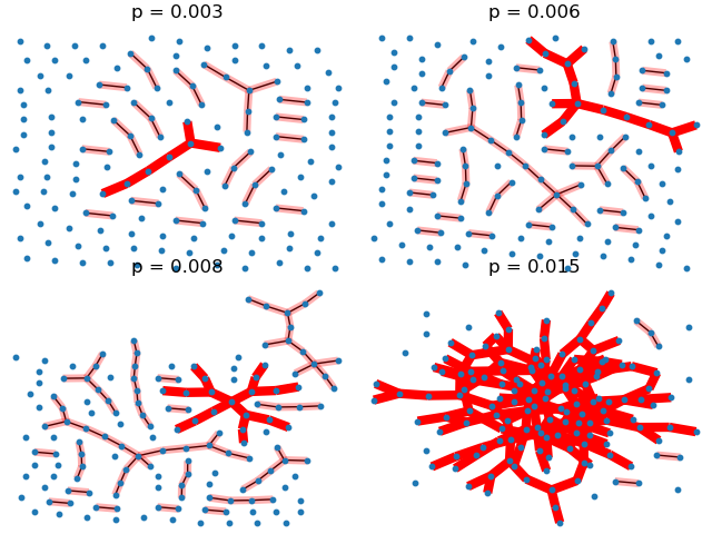
Giant Component
This example illustrates the sudden appearance of a giant connected component in a binomial random graph.
import math

import matplotlib.pyplot as plt
import networkx as nx

# This example needs Graphviz and either PyGraphviz or pydot.
# from networkx.drawing.nx_pydot import graphviz_layout as layout
from networkx.drawing.nx_agraph import graphviz_layout as layout

# If you don't have pygraphviz or pydot, you can do this
# layout = nx.spring_layout


n = 150  # 150 nodes
# p value at which giant component (of size log(n) nodes) is expected
p_giant = 1.0 / (n - 1)
# p value at which graph is expected to become completely connected
p_conn = math.log(n) / float(n)

# the following range of p values should be close to the threshold
pvals = [0.003, 0.006, 0.008, 0.015]

region = 220  # for pylab 2x2 subplot layout
plt.subplots_adjust(left=0, right=1, bottom=0, top=0.95, wspace=0.01, hspace=0.01)
for p in pvals:
    G = nx.binomial_graph(n, p)
    pos = layout(G)
    region += 1
    plt.subplot(region)
    plt.title(f"p = {p:.3f}")
    nx.draw(G, pos, with_labels=False, node_size=10)
    # identify largest connected component
    Gcc = sorted(nx.connected_components(G), key=len, reverse=True)
    G0 = G.subgraph(Gcc[0])
    nx.draw_networkx_edges(G0, pos, edge_color="r", width=6.0)
    # show other connected components
    for Gi in Gcc[1:]:
        if len(Gi) > 1:
            nx.draw_networkx_edges(
                G.subgraph(Gi), pos, edge_color="r", alpha=0.3, width=5.0,
            )
plt.show()
Total running time of the script: ( 0 minutes 0.958 seconds)