What's new in Matplotlib 3.4.0 (Mar 26, 2021)#
For a list of all of the issues and pull requests since the last revision, see the GitHub statistics for 3.10.1 (Feb 27, 2025).
Figure and Axes creation / management#
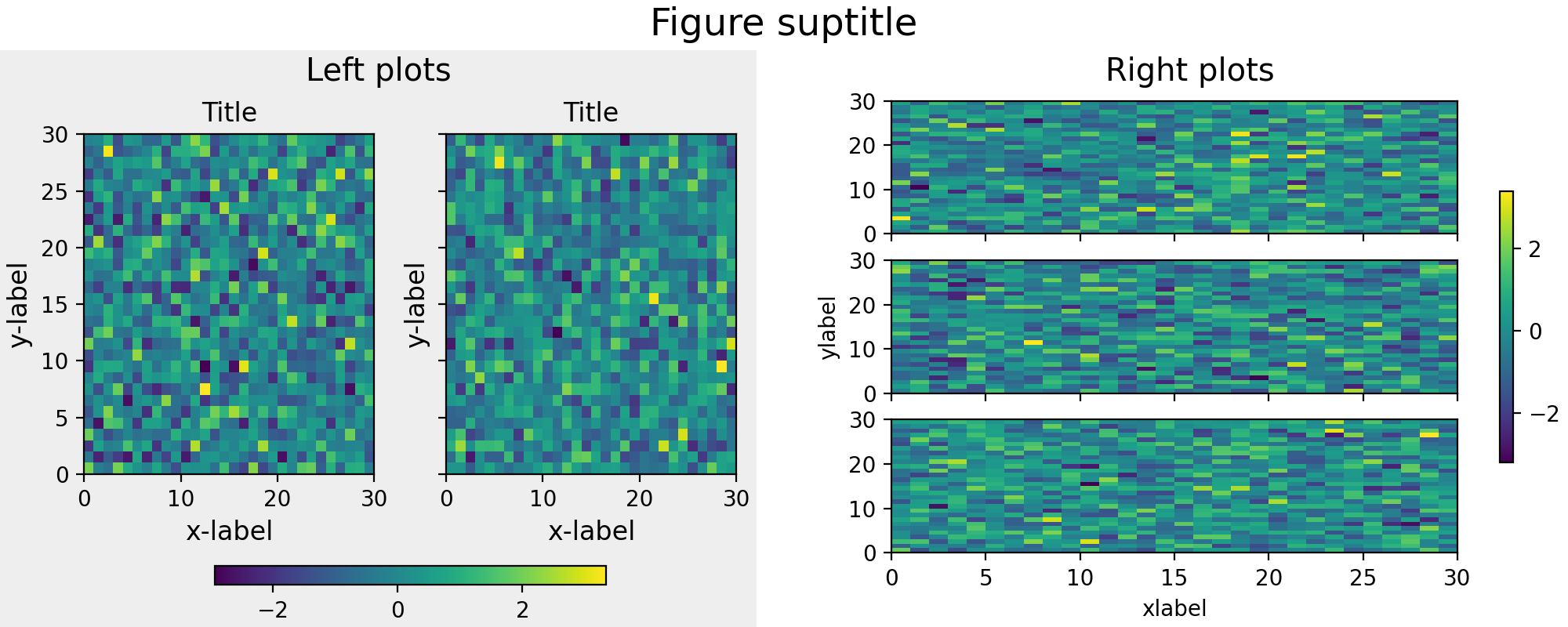
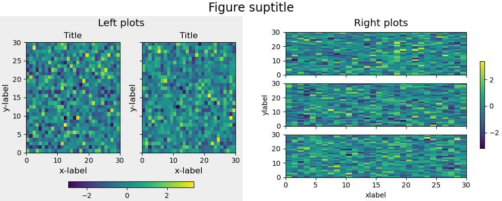
New subfigure functionality#
New figure.Figure.add_subfigure and figure.Figure.subfigures
functionalities allow creating virtual figures within figures. Similar nesting
was previously done with nested gridspecs (see
Nested Gridspecs). However, this did
not allow localized figure artists (e.g., a colorbar or suptitle) that only
pertained to each subgridspec.
The new methods figure.Figure.add_subfigure and figure.Figure.subfigures
are meant to rhyme with figure.Figure.add_subplot and
figure.Figure.subplots and have most of the same arguments.
See Figure subfigures for further details.
Note
The subfigure functionality is experimental API as of v3.4.
(Source code, 2x.png, png)

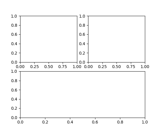
Single-line string notation for subplot_mosaic#
Figure.subplot_mosaic and pyplot.subplot_mosaic now accept a single-line
string, using semicolons to delimit rows. Namely,
plt.subplot_mosaic(
    """
    AB
    CC
    """)
may be written as the shorter:
plt.subplot_mosaic("AB;CC")
(Source code, 2x.png, png)

Changes to behavior of Axes creation methods (gca, add_axes, add_subplot)#
The behavior of the functions to create new Axes (pyplot.axes,
pyplot.subplot, figure.Figure.add_axes, figure.Figure.add_subplot) has
changed. In the past, these functions would detect if you were attempting to
create Axes with the same keyword arguments as already-existing Axes in the
current Figure, and if so, they would return the existing Axes. Now,
pyplot.axes, figure.Figure.add_axes, and figure.Figure.add_subplot
will always create new Axes. pyplot.subplot will continue to reuse an
existing Axes with a matching subplot spec and equal kwargs.
Correspondingly, the behavior of the functions to get the current Axes
(pyplot.gca, figure.Figure.gca) has changed. In the past, these functions
accepted keyword arguments. If the keyword arguments matched an
already-existing Axes, then that Axes would be returned, otherwise new Axes
would be created with those keyword arguments. Now, the keyword arguments are
only considered if there are no Axes at all in the current figure. In a future
release, these functions will not accept keyword arguments at all.
add_subplot/add_axes gained an axes_class parameter#
In particular, mpl_toolkits Axes subclasses can now be idiomatically used
using, e.g., fig.add_subplot(axes_class=mpl_toolkits.axislines.Axes)
Subplot and subplot2grid can now work with constrained layout#
constrained_layout depends on a single GridSpec for each logical layout
on a figure. Previously, pyplot.subplot and pyplot.subplot2grid added a
new GridSpec each time they were called and were therefore incompatible
with constrained_layout.
Now subplot attempts to reuse the GridSpec if the number of rows and
columns is the same as the top level GridSpec already in the figure, i.e.,
plt.subplot(2, 1, 2) will use the same GridSpec as plt.subplot(2, 1, 1)
and the constrained_layout=True option to Figure will work.
In contrast, mixing nrows and ncols will not work with
constrained_layout: plt.subplot(2, 2, 1) followed by plt.subplots(2,
1, 2) will still produce two GridSpecs, and constrained_layout=True will
give bad results. In order to get the desired effect, the second call can
specify the cells the second Axes is meant to cover: plt.subplots(2, 2, (2,
4)), or the more Pythonic plt.subplot2grid((2, 2), (0, 1), rowspan=2) can
be used.
Plotting methods#
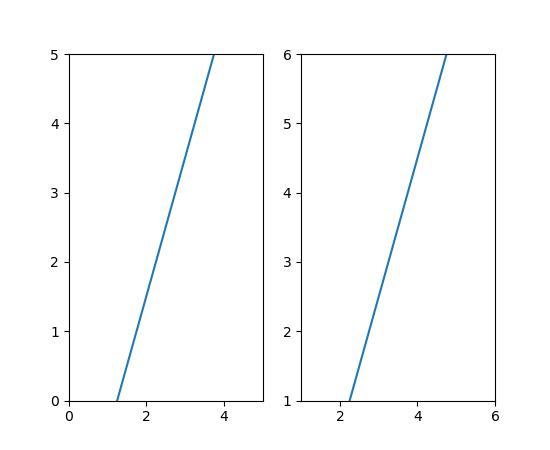
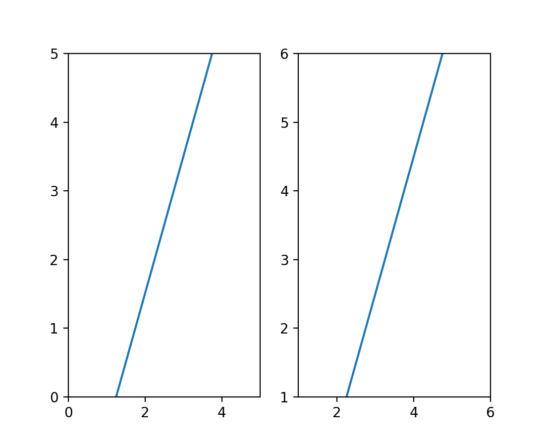
axline supports transform parameter#
axline now supports the transform parameter, which applies to the
points xy1, xy2. The slope (if given) is always in data coordinates.
For example, this can be used with ax.transAxes for drawing lines with a
fixed slope. In the following plot, the line appears through the same point on
both Axes, even though they show different data limits.
fig, axs = plt.subplots(1, 2)

for i, ax in enumerate(axs):
    ax.axline((0.25, 0), slope=2, transform=ax.transAxes)
    ax.set(xlim=(i, i+5), ylim=(i, i+5))
(Source code, 2x.png, png)
New automatic labeling for bar charts#
A new Axes.bar_label method has been added for auto-labeling bar charts.
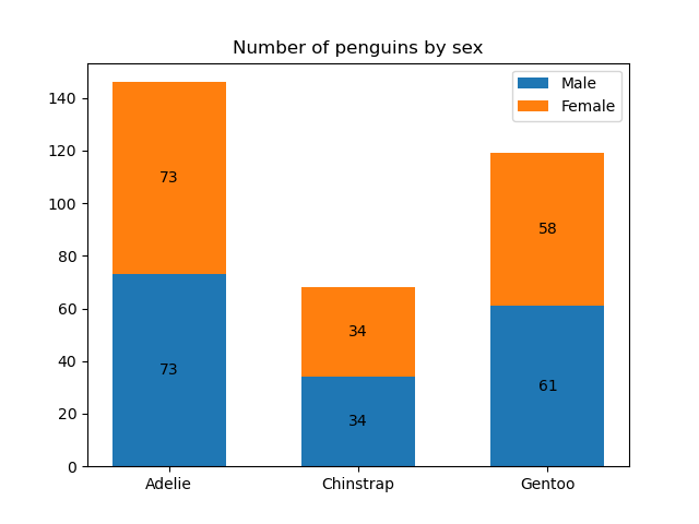
Example of the new automatic labeling.#
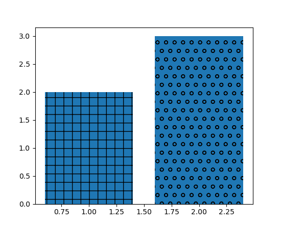
A list of hatches can be specified to bar and barh#
Similar to some other rectangle properties, it is now possible to hand a list
of hatch styles to bar and barh in order to create
bars with different hatch styles, e.g.
(Source code, 2x.png, png)

Setting BarContainer orientation#
BarContainer now accepts a new string argument orientation. It can be
either 'vertical' or 'horizontal', default is None.
Contour plots now default to using ScalarFormatter#
Pass fmt="%1.3f" to the contouring call to restore the old default label
format.
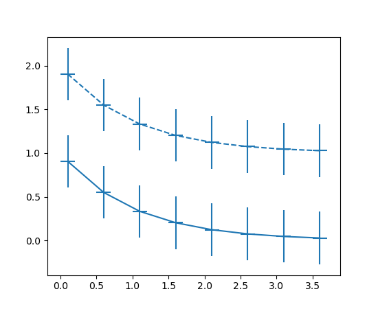
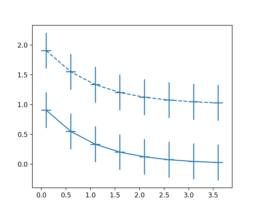
Axes.errorbar cycles non-color properties correctly#
Formerly, Axes.errorbar incorrectly skipped the Axes property cycle if a
color was explicitly specified, even if the property cycler was for other
properties (such as line style). Now, Axes.errorbar will advance the Axes
property cycle as done for Axes.plot, i.e., as long as all properties in the
cycler are not explicitly passed.
For example, the following will cycle through the line styles:
x = np.arange(0.1, 4, 0.5)
y = np.exp(-x)
offsets = [0, 1]

plt.rcParams['axes.prop_cycle'] = plt.cycler('linestyle', ['-', '--'])

fig, ax = plt.subplots()
for offset in offsets:
    ax.errorbar(x, y + offset, xerr=0.1, yerr=0.3, fmt='tab:blue')
(Source code, 2x.png, png)
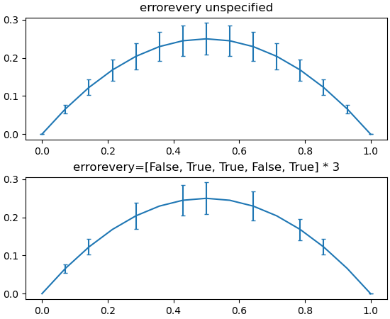
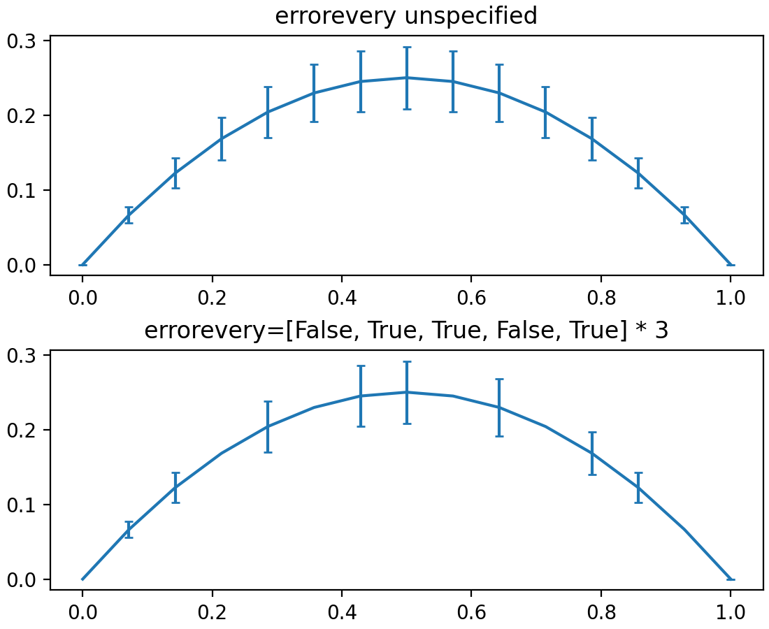
errorbar errorevery parameter matches markevery#
Similar to the markevery parameter to plot, the errorevery
parameter of errorbar now accept slices and NumPy fancy indexes (which
must match the size of x).
(Source code, 2x.png, png)
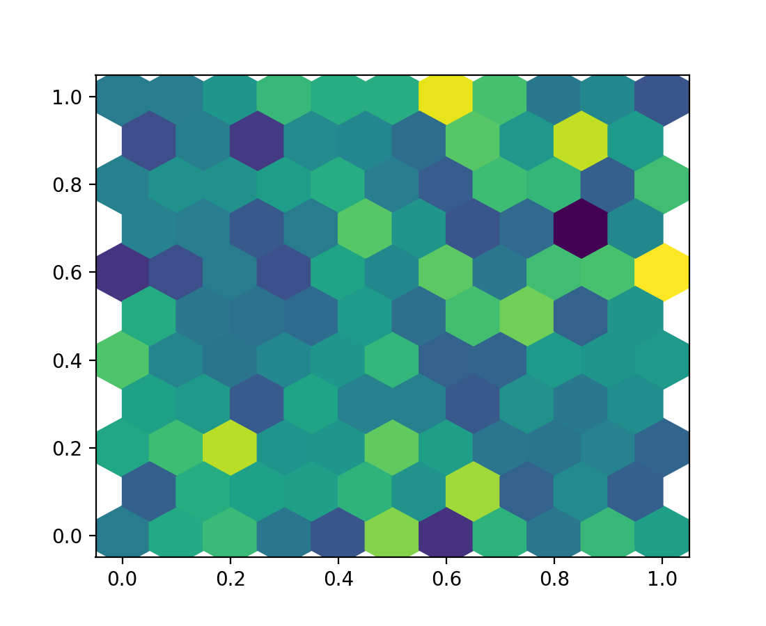
hexbin supports data reference for C parameter#
As with the x and y parameters, Axes.hexbin now supports passing the C
parameter using a data reference.
data = {
    'a': np.random.rand(1000),
    'b': np.random.rand(1000),
    'c': np.random.rand(1000),
}

fig, ax = plt.subplots()
ax.hexbin('a', 'b', C='c', data=data, gridsize=10)
(Source code, 2x.png, png)

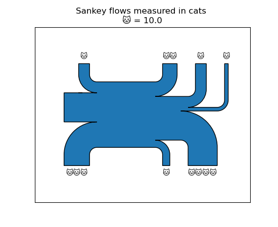
Support callable for formatting of Sankey labels#
The format parameter of matplotlib.sankey.Sankey can now accept callables.
This allows the use of an arbitrary function to label flows, for example allowing the mapping of numbers to emoji.
(Source code, 2x.png, png)

Axes.spines access shortcuts#
Axes.spines is now a dedicated container class Spines for a set of
Spines instead of an OrderedDict. On top of dict-like access,
Axes.spines now also supports some pandas.Series-like features.
Accessing single elements by item or by attribute:
ax.spines['top'].set_visible(False)
ax.spines.top.set_visible(False)
Accessing a subset of items:
ax.spines[['top', 'right']].set_visible(False)
Accessing all items simultaneously:
ax.spines[:].set_visible(False)
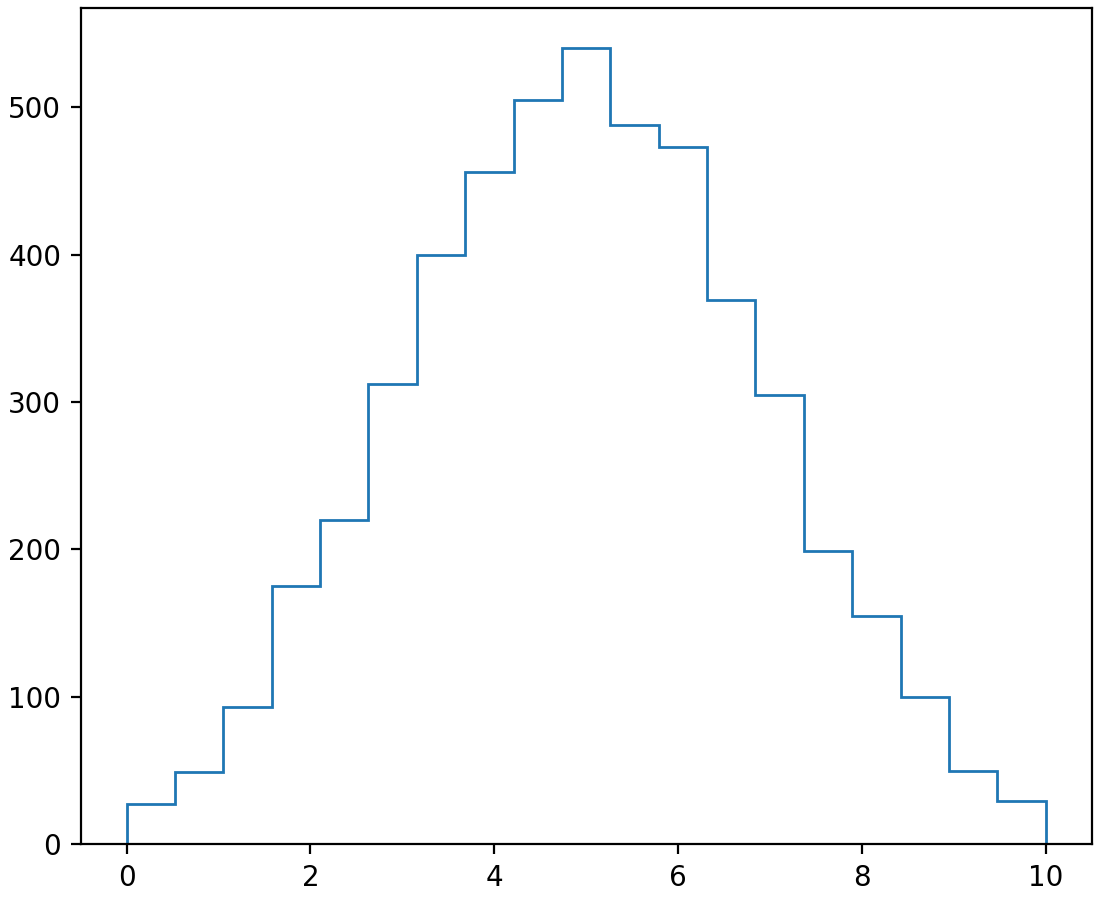
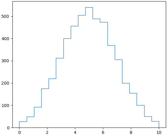
New stairs method and StepPatch artist#
pyplot.stairs and the underlying artist StepPatch
provide a cleaner interface for plotting stepwise constant functions for the
common case that you know the step edges. This supersedes many use cases of
pyplot.step, for instance when plotting the output of numpy.histogram.
For both the artist and the function, the x-like edges input is one element longer than the y-like values input
(Source code, 2x.png, png)

See Stairs Demo for examples.
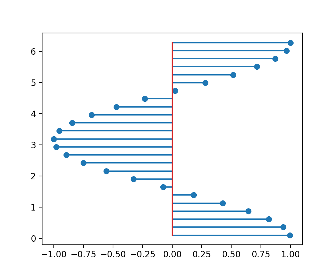
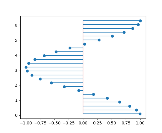
Added orientation parameter for stem plots#
By default, stem lines are vertical. They can be changed to horizontal using
the orientation parameter of Axes.stem or pyplot.stem:
(Source code, 2x.png, png)

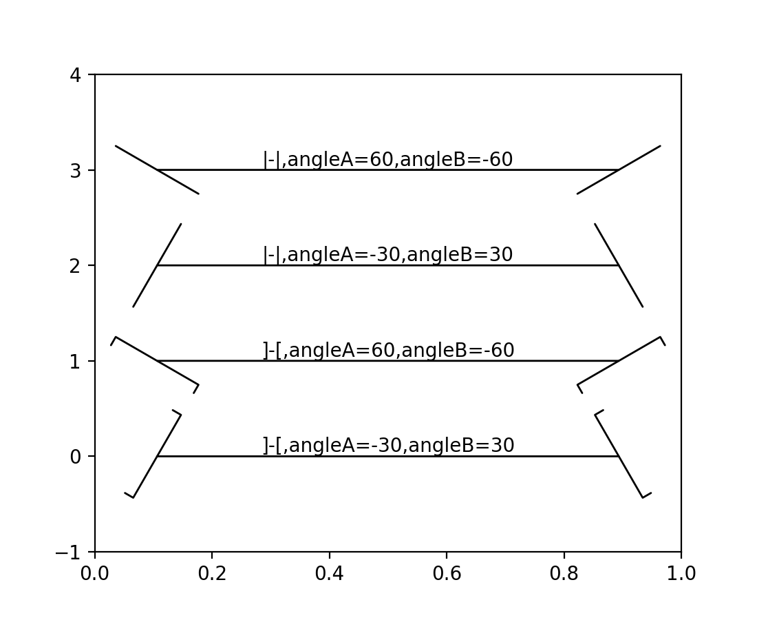
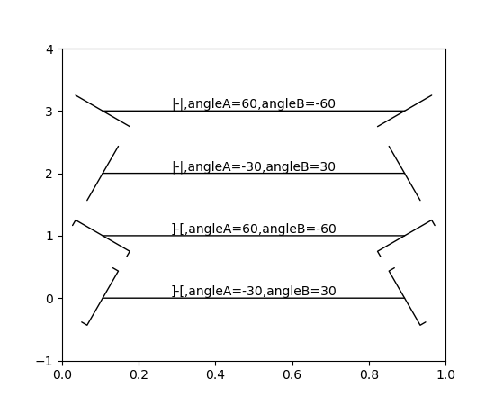
Angles on Bracket arrow styles#
Angles specified on the Bracket arrow styles (]-[, ]-, -[, or
|-| passed to arrowstyle parameter of FancyArrowPatch) are now
applied. Previously, the angleA and angleB options were allowed, but did
nothing.
(Source code, 2x.png, png)

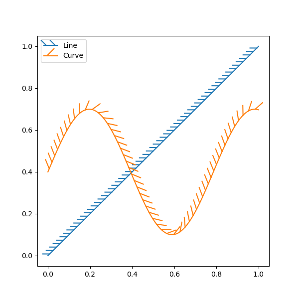
TickedStroke patheffect#
The new TickedStroke patheffect can be used to produce lines with a ticked
style. This can be used to, e.g., distinguish the valid and invalid sides of
the constraint boundaries in the solution space of optimizations.
Colors and colormaps#
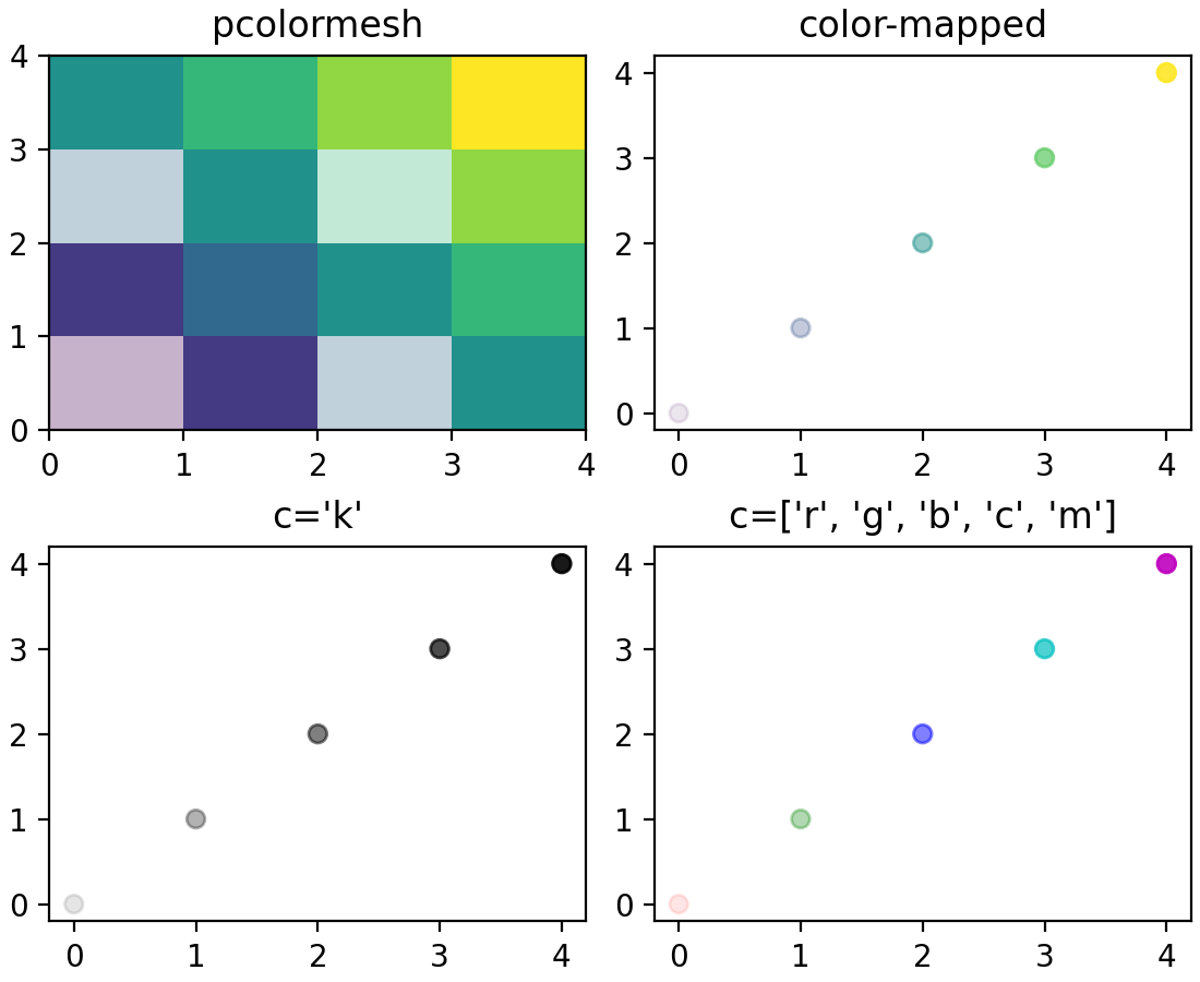
Collection color specification and mapping#
Reworking the handling of color mapping and the keyword arguments for facecolor and edgecolor has resulted in three behavior changes:
Color mapping can be turned off by calling
Collection.set_array(None). Previously, this would have no effect.When a mappable array is set, with
facecolor='none'andedgecolor='face', both the faces and the edges are left uncolored. Previously the edges would be color-mapped.When a mappable array is set, with
facecolor='none'andedgecolor='red', the edges are red. This addresses Issue #1302. Previously the edges would be color-mapped.
Transparency (alpha) can be set as an array in collections#
Previously, the alpha value controlling transparency in collections could be
specified only as a scalar applied to all elements in the collection. For
example, all the markers in a scatter plot, or all the quadrilaterals
in a pcolormesh plot, would have the same alpha value.
Now it is possible to supply alpha as an array with one value for each element (marker, quadrilateral, etc.) in a collection.
(Source code, 2x.png, png)

pcolormesh has improved transparency handling by enabling snapping#
Due to how the snapping keyword argument was getting passed to the Agg backend,
previous versions of Matplotlib would appear to show lines between the grid
edges of a mesh with transparency. This version now applies snapping by
default. To restore the old behavior (e.g., for test images), you may set
rcParams["pcolormesh.snap"] (default: True) to False.
(Source code, 2x.png, png)
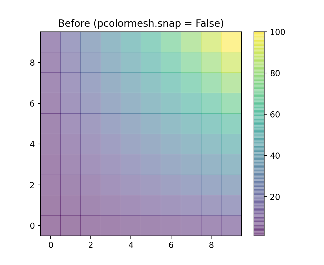
Note that there are lines between the grid boundaries of the main plot which are not the same transparency. The colorbar also shows these lines when a transparency is added to the colormap because internally it uses pcolormesh to draw the colorbar. With snapping on by default (below), the lines at the grid boundaries disappear.
(Source code, 2x.png, png)

IPython representations for Colormap objects#
The matplotlib.colors.Colormap object now has image representations for
IPython / Jupyter backends. Cells returning a colormap on the last line will
display an image of the colormap.
In[1]: cmap = plt.get_cmap('viridis').with_extremes(bad='r', under='g', over='b')

In[2]: cmap
Out[2]:

Colormap.set_extremes and Colormap.with_extremes#
Because the Colormap.set_bad, Colormap.set_under and Colormap.set_over
methods modify the colormap in place, the user must be careful to first make a
copy of the colormap if setting the extreme colors e.g. for a builtin colormap.
The new Colormap.with_extremes(bad=..., under=..., over=...) can be used to
first copy the colormap and set the extreme colors on that copy.
The new Colormap.set_extremes method is provided for API symmetry with
Colormap.with_extremes, but note that it suffers from the same issue as the
earlier individual setters.
Get under/over/bad colors of Colormap objects#
matplotlib.colors.Colormap now has methods get_under,
get_over, get_bad for the colors used
for out-of-range and masked values.
New cm.unregister_cmap function#
matplotlib.cm.unregister_cmap allows users to remove a colormap that they have
previously registered.
New CenteredNorm for symmetrical data around a center#
In cases where data is symmetrical around a center, for example, positive and
negative anomalies around a center zero, CenteredNorm is
a new norm that automatically creates a symmetrical mapping around the center.
This norm is well suited to be combined with a divergent colormap which uses an
unsaturated color in its center.
(Source code, 2x.png, png)
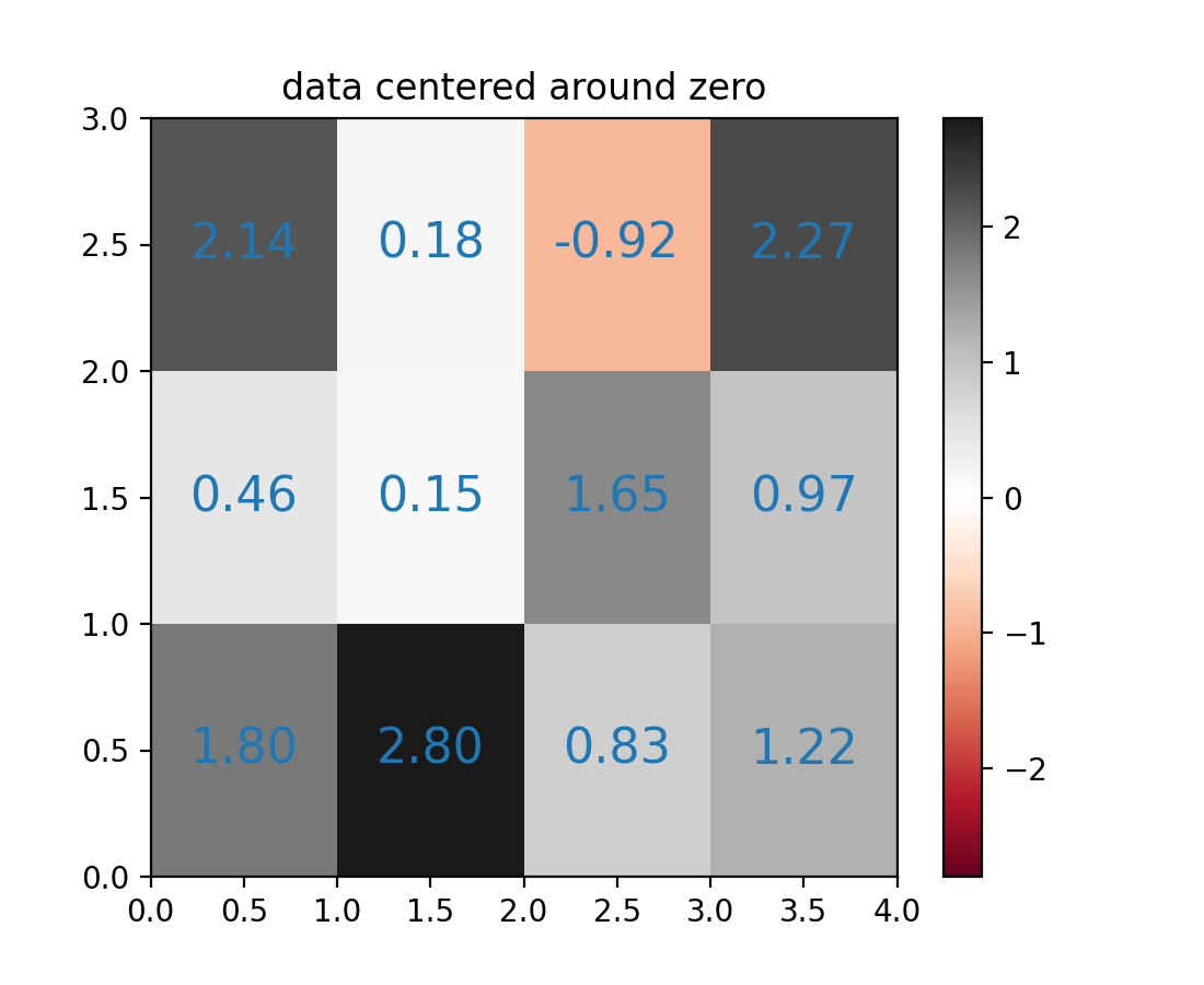
If the center of symmetry is different from 0, it can be set with the vcenter
argument. To manually set the range of CenteredNorm, use
the halfrange argument.
See Colormap normalization for an example and more details about data normalization.
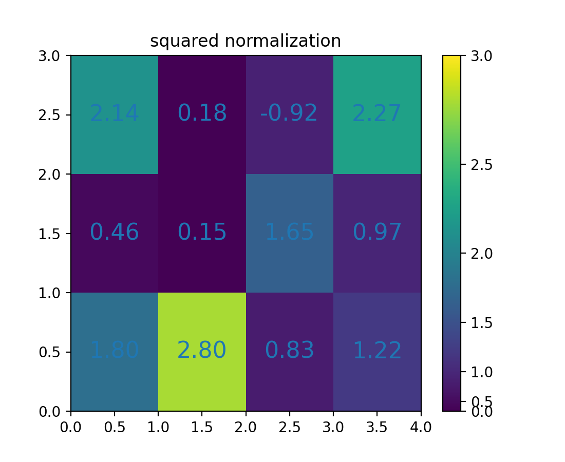
New FuncNorm for arbitrary normalizations#
The FuncNorm allows for arbitrary normalization using functions for the
forward and inverse.
(Source code, 2x.png, png)

See Colormap normalization for an example and more details about data normalization.
GridSpec-based colorbars can now be positioned above or to the left of the main axes#
... by passing location="top" or location="left" to the colorbar()
call.
Titles, ticks, and labels#
supxlabel and supylabel#
It is possible to add x- and y-labels to a whole figure, analogous to
Figure.suptitle using the new Figure.supxlabel and
Figure.supylabel methods.
(Source code, 2x.png, png)

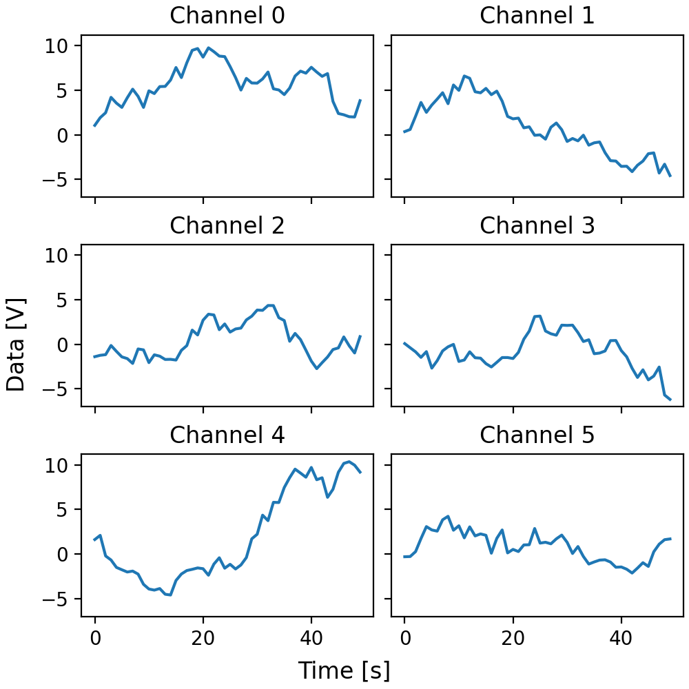
Shared-axes subplots tick label visibility is now correct for top or left labels#
When calling subplots(..., sharex=True, sharey=True), Matplotlib
automatically hides x tick labels for Axes not in the first column and y tick
labels for Axes not in the last row. This behavior is incorrect if rcParams
specify that Axes should be labeled on the top (rcParams["xtick.labeltop"] =
True) or on the right (rcParams["ytick.labelright"] = True).
Cases such as the following are now handled correctly (adjusting visibility as needed on the first row and last column of Axes):
plt.rcParams["xtick.labelbottom"] = False
plt.rcParams["xtick.labeltop"] = True
plt.rcParams["ytick.labelleft"] = False
plt.rcParams["ytick.labelright"] = True

fig, axs = plt.subplots(2, 2, sharex=True, sharey=True)
(Source code, 2x.png, png)
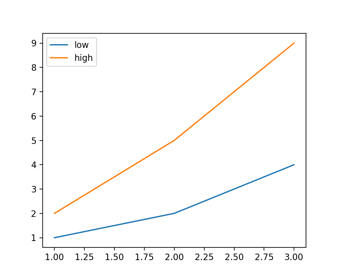
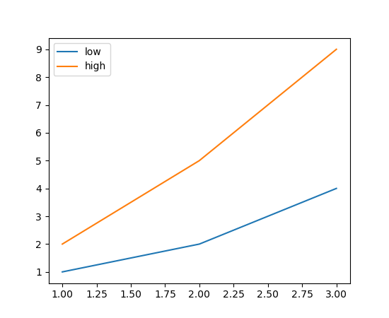
An iterable object with labels can be passed to Axes.plot#
When plotting multiple datasets by passing 2D data as y value to
plot, labels for the datasets can be passed as a list, the length
matching the number of columns in y.
x = [1, 2, 3]

y = [[1, 2],
     [2, 5],
     [4, 9]]

plt.plot(x, y, label=['low', 'high'])
plt.legend()
(Source code, 2x.png, png)

Fonts and Text#
Text transform can rotate text direction#
The new Text parameter transform_rotates_text now sets whether rotations
of the transform affect the text direction.
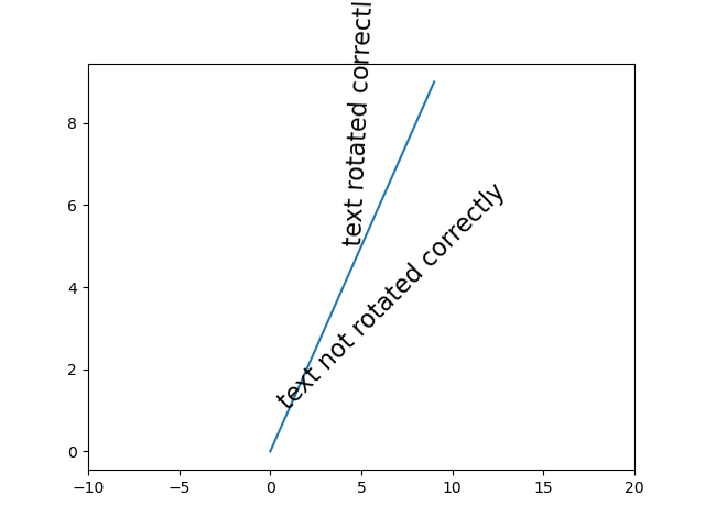
Example of the new transform_rotates_text parameter#
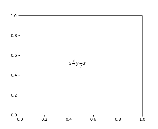
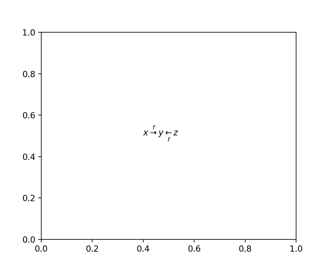
matplotlib.mathtext now supports overset and underset LaTeX symbols#
mathtext now supports overset and underset, called as
\overset{annotation}{body} or \underset{annotation}{body}, where
annotation is the text "above" or "below" the body.
(Source code, 2x.png, png)
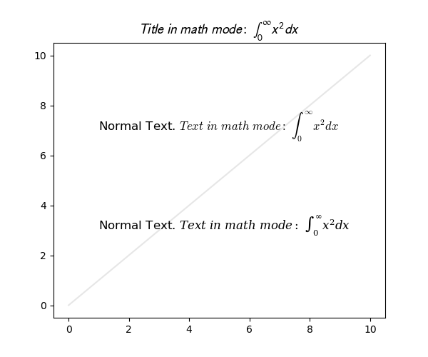
math_fontfamily parameter to change Text font family#
The new math_fontfamily parameter may be used to change the family of fonts
for each individual text element in a plot. If no parameter is set, the global
value rcParams["mathtext.fontset"] (default: 'dejavusans') will be used.
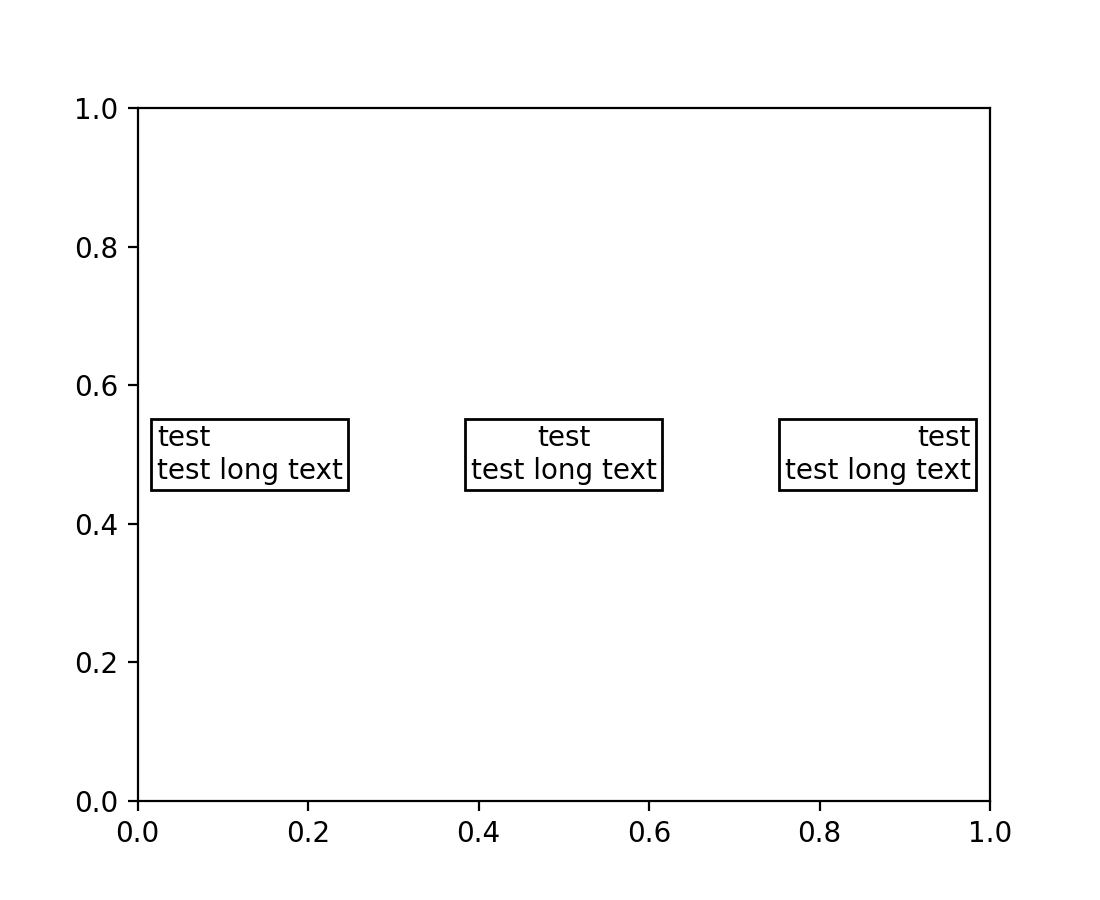
TextArea/AnchoredText support horizontalalignment#
The horizontal alignment of text in a TextArea or AnchoredText may now be
specified, which is mostly effective for multiline text:
(Source code, 2x.png, png)

PDF supports URLs on Text artists#
URLs on text.Text artists (i.e., from Artist.set_url) will now be saved
in PDF files.
rcParams improvements#
New rcParams for dates: set converter and whether to use interval_multiples#
The new rcParams["date.converter"] (default: 'auto') allows toggling between
matplotlib.dates.DateConverter and matplotlib.dates.ConciseDateConverter
using the strings 'auto' and 'concise' respectively.
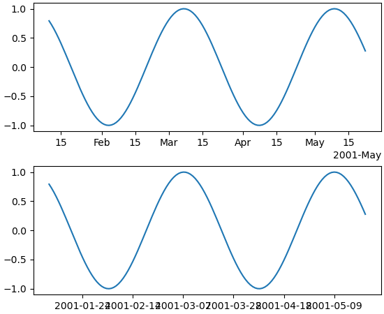
The new rcParams["date.interval_multiples"] (default: True) allows toggling between the dates locator
trying to pick ticks at set intervals (i.e., day 1 and 15 of the month), versus
evenly spaced ticks that start wherever the timeseries starts:
dates = np.arange('2001-01-10', '2001-05-23', dtype='datetime64[D]')
y = np.sin(dates.astype(float) / 10)
fig, axs = plt.subplots(nrows=2, constrained_layout=True)

plt.rcParams['date.converter'] = 'concise'
plt.rcParams['date.interval_multiples'] = True
axs[0].plot(dates, y)

plt.rcParams['date.converter'] = 'auto'
plt.rcParams['date.interval_multiples'] = False
axs[1].plot(dates, y)
(Source code, 2x.png, png)

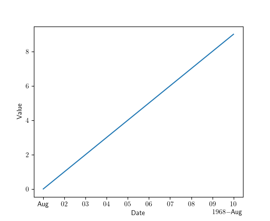
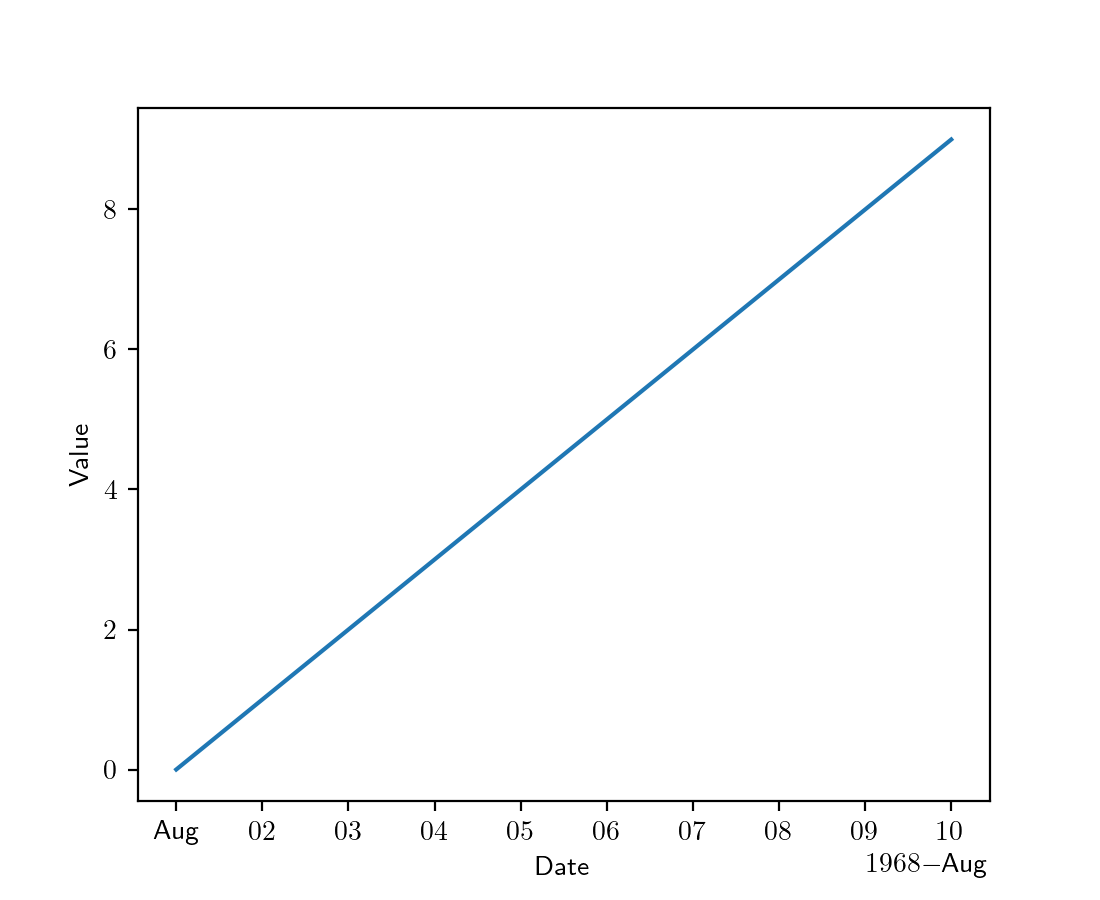
Date formatters now respect usetex rcParam#
The AutoDateFormatter and ConciseDateFormatter now respect
rcParams["text.usetex"] (default: False), and will thus use fonts consistent with TeX rendering of the
default (non-date) formatter. TeX rendering may also be enabled/disabled by
passing the usetex parameter when creating the formatter instance.
In the following plot, both the x-axis (dates) and y-axis (numbers) now use the same (TeX) font:
(Source code, 2x.png, png)
Setting image.cmap to a Colormap#
It is now possible to set rcParams["image.cmap"] (default: 'viridis') to a Colormap instance, such as a
colormap created with the new set_extremes above. (This can only
be done from Python code, not from the matplotlibrc file.)
Tick and tick label colors can be set independently using rcParams#
Previously, rcParams["xtick.color"] (default: 'black') defined both the tick color and the label color.
The label color can now be set independently using rcParams["xtick.labelcolor"] (default: 'inherit'). It
defaults to 'inherit' which will take the value from rcParams["xtick.color"] (default: 'black'). The
same holds for ytick.[label]color. For instance, to set the ticks to light
grey and the tick labels to black, one can use the following code in a script:
import matplotlib as mpl

mpl.rcParams['xtick.labelcolor'] = 'lightgrey'
mpl.rcParams['xtick.color'] = 'black'
mpl.rcParams['ytick.labelcolor'] = 'lightgrey'
mpl.rcParams['ytick.color'] = 'black'
Or by adding the following lines to the matplotlibrc file, or a Matplotlib style file:
xtick.labelcolor : lightgrey
xtick.color      : black
ytick.labelcolor : lightgrey
ytick.color      : black
3D Axes improvements#
Errorbar method in 3D Axes#
The errorbar function Axes.errorbar is ported into the 3D Axes framework in
its entirety, supporting features such as custom styling for error lines and
cap marks, control over errorbar spacing, upper and lower limit marks.

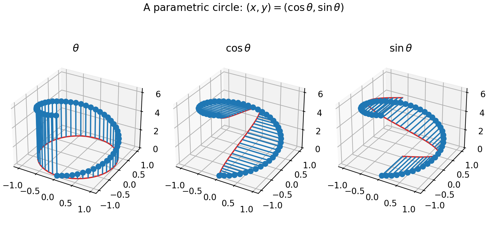
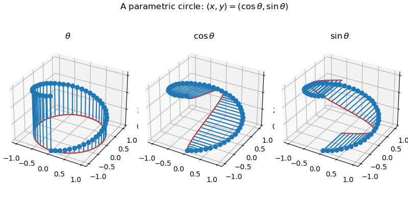
Stem plots in 3D Axes#
Stem plots are now supported on 3D Axes. Much like 2D stems,
stem supports plotting the stems in various orientations:
(Source code, 2x.png, png)

See also the 3D stem demo.
3D Collection properties are now modifiable#
Previously, properties of a 3D Collection that were used for 3D effects (e.g., colors were modified to produce depth shading) could not be changed after it was created.
Now it is possible to modify all properties of 3D Collections at any time.
Panning in 3D Axes#
Click and drag with the middle mouse button to pan 3D Axes.
Interactive tool improvements#
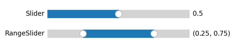
New RangeSlider widget#
widgets.RangeSlider allows for creating a slider that defines
a range rather than a single value.
(Source code, 2x.png, png)

Sliders can now snap to arbitrary values#
The Slider UI widget now accepts arrays for valstep.
This generalizes the previous behavior by allowing the slider to snap to
arbitrary values.
Pausing and Resuming Animations#
The animation.Animation.pause and animation.Animation.resume methods
allow you to pause and resume animations. These methods can be used as
callbacks for event listeners on UI elements so that your plots can have some
playback control UI.
Sphinx extensions#
plot_directive caption option#
Captions were previously supported when using the plot_directive directive
with an external source file by specifying content:
.. plot:: path/to/plot.py

    This is the caption for the plot.
The :caption: option allows specifying the caption for both external:
.. plot:: path/to/plot.py
    :caption: This is the caption for the plot.
and inline plots:
.. plot::
    :caption: This is a caption for the plot.

    plt.plot([1, 2, 3])
Backend-specific improvements#
Consecutive rasterized draws now merged#
Elements of a vector output can be individually set to rasterized, using the
rasterized keyword argument, or set_rasterized(). This can
be useful to reduce file sizes. For figures with multiple raster elements they
are now automatically merged into a smaller number of bitmaps where this will
not effect the visual output. For cases with many elements this can result in
significantly smaller file sizes.
To ensure this happens do not place vector elements between raster ones.
To inhibit this merging set Figure.suppressComposite to True.
Support raw/rgba frame format in FFMpegFileWriter#
When using FFMpegFileWriter, the frame_format may now be set to "raw"
or "rgba", which may be slightly faster than an image format, as no
encoding/decoding need take place between Matplotlib and FFmpeg.
nbAgg/WebAgg support middle-click and double-click#
Double click events are now supported by the nbAgg and WebAgg backends. Formerly, WebAgg would report middle-click events as right clicks, but now reports the correct button type.
nbAgg support binary communication#
If the web browser and notebook support binary websockets, nbAgg will now use them for slightly improved transfer of figure display.
Indexed color for PNG images in PDF files when possible#
When PNG images have 256 colors or fewer, they are converted to indexed color before saving them in a PDF. This can result in a significant reduction in file size in some cases. This is particularly true for raster data that uses a colormap but no interpolation, such as Healpy mollview plots. Currently, this is only done for RGB images.
Improved font subsettings in PDF/PS#
Font subsetting in PDF and PostScript has been re-written from the embedded
ttconv C code to Python. Some composite characters and outlines may have
changed slightly. This fixes ttc subsetting in PDF, and adds support for
subsetting of type 3 OTF fonts, resulting in smaller files (much smaller when
using CJK fonts), and avoids running into issues with type 42 embedding and
certain PDF readers such as Acrobat Reader.
Kerning added to strings in PDFs#
As with text produced in the Agg backend (see the previous what's new entry for examples), PDFs now include kerning in text strings.
Fully-fractional HiDPI in QtAgg#
Fully-fractional HiDPI (that is, HiDPI ratios that are not whole integers) was added in Qt 5.14, and is now supported by the QtAgg backend when using this version of Qt or newer.
wxAgg supports fullscreen toggle#
The wxAgg backend supports toggling fullscreen using the f shortcut, or
the manager function FigureManagerBase.full_screen_toggle.