

Data Tables (astropy.table)#
Introduction#
astropy.table provides a flexible and easy-to-use set of tools for working with
tabular data using an interface based on numpy. In addition to basic table creation,
access, and modification operations, key features include:
Support columns of astropy time, coordinates, and quantities.
Support multidimensional and structured array columns.
Maintain the units, description, and format of columns.
Provide flexible metadata structures for the table and individual columns.
Perform Table Operations like database joins, concatenation, and binning.
Maintain a table index for fast retrieval of table items or ranges.
Support a general mixin protocol for flexible data containers in tables.
Read and write to files via the Unified File Read/Write Interface.
Convert to and from
pandas.DataFrame.
The Astropy Table and DataFrames page provides the rationale for maintaining
and using the dedicated astropy.table package instead of relying on pandas.
Getting Started#
The basic workflow for creating a table, accessing table elements,
and modifying the table is shown below. These examples demonstrate a concise
case, while the full astropy.table documentation is available from the
Using table section.
First create a simple table with columns of data named a, b, c, and
d. These columns have integer, float, string, and |Quantity| values
respectively:
>>> from astropy.table import QTable
>>> import astropy.units as u
>>> import numpy as np

>>> a = np.array([1, 4, 5], dtype=np.int32)
>>> b = [2.0, 5.0, 8.5]
>>> c = ['x', 'y', 'z']
>>> d = [10, 20, 30] * u.m / u.s

>>> t = QTable([a, b, c, d],
...            names=('a', 'b', 'c', 'd'),
...            meta={'name': 'first table'})
Comments:
Column
ais a |ndarray| with a specifieddtypeofint32. If the data type is not provided, the default type for integers isint64on Mac and Linux andint32on Windows.Column
bis a list offloatvalues, represented asfloat64.Column
cis a list ofstrvalues, represented as unicode. See Bytestring Columns for more information.Column
dis a |Quantity| array. Since we used |QTable|, this stores a native |Quantity| within the table and brings the full power of Units and Quantities (astropy.units) to this column in the table.
Note
If the table data have no units or you prefer to not use |Quantity|, then you can use the |Table| class to create tables. The only difference between |QTable| and |Table| is the behavior when adding a column that has units. See Quantity and QTable and Columns with Units for details on the differences and use cases.
There are many other ways of Constructing a Table, including from a list of
rows (either tuples or dicts), from a numpy structured or 2D array, by
adding columns or rows incrementally, or even converting from a |SkyCoord| or a
pandas.DataFrame.
There are a few ways of Accessing a Table. You can get detailed information about the table values and column definitions as follows:
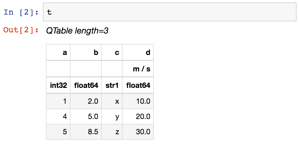
>>> t
<QTable length=3>
  a      b     c      d
                    m / s
int32 float64 str1 float64
----- ------- ---- -------
    1     2.0    x    10.0
    4     5.0    y    20.0
    5     8.5    z    30.0
You can get summary information about the table as follows:
>>> t.info
<QTable length=3>
name  dtype   unit  class
---- ------- ----- --------
   a   int32         Column
   b float64         Column
   c    str1         Column
   d float64 m / s Quantity
From within a Jupyter notebook, the table is
displayed as a formatted HTML table (details of how it appears can be changed
by altering the astropy.table.conf.default_notebook_table_class item in the
Configuration System (astropy.config):
Or you can get a fancier notebook interface with show_in_notebook(),
e.g., when used with backend="ipydatagrid", it comes with in-browser filtering and sort:
If you print the table (either from the notebook or in a text console session) then a formatted version appears:
>>> print(t)
 a   b   c    d
            m / s
--- --- --- -----
  1 2.0   x  10.0
  4 5.0   y  20.0
  5 8.5   z  30.0
If you do not like the format of a particular column, you can change it through the ‘info’ property:
>>> t['b'].info.format = '7.3f'
>>> print(t)
 a     b     c    d
                m / s
--- ------- --- -----
  1   2.000   x  10.0
  4   5.000   y  20.0
  5   8.500   z  30.0
For a long table you can scroll up and down through the table one page at time:
>>> t.more()
You can also display it as an HTML-formatted table in the browser:
>>> t.show_in_browser()
Or as an interactive (searchable and sortable) javascript table:
>>> t.show_in_browser(jsviewer=True)
Now examine some high-level information about the table:
>>> t.colnames
['a', 'b', 'c', 'd']
>>> len(t)
3
>>> t.meta
{'name': 'first table'}
Access the data by column or row using familiar numpy structured array
syntax:
>>> t['a']       # Column 'a'
<Column name='a' dtype='int32' length=3>
1
4
5

>>> t['a'][1]    # Row 1 of column 'a'
np.int32(4)

>>> t[1]         # Row 1 of the table
<Row index=1>
  a      b     c      d
                    m / s
int32 float64 str1 float64
----- ------- ---- -------
    4   5.000    y    20.0


>>> t[1]['a']    # Column 'a' of row 1
np.int32(4)
You can retrieve a subset of a table by rows (using a slice) or by
columns (using column names), where the subset is returned as a new table:
>>> print(t[0:2])      # Table object with rows 0 and 1
 a     b     c    d
                m / s
--- ------- --- -----
  1   2.000   x  10.0
  4   5.000   y  20.0


>>> print(t['a', 'c'])  # Table with cols 'a' and 'c'
 a   c
--- ---
  1   x
  4   y
  5   z
Modifying a Table in place is flexible and works as you would expect:
>>> t['a'][:] = [-1, -2, -3]    # Set all column values in place
>>> t['a'][2] = 30              # Set row 2 of column 'a'
>>> t[1] = (8, 9.0, "W", 4 * u.m / u.s) # Set all values of row 1
>>> t[1]['b'] = -9              # Set column 'b' of row 1
>>> t[0:2]['b'] = 100.0         # Set column 'b' of rows 0 and 1
>>> print(t)
 a     b     c    d
                m / s
--- ------- --- -----
 -1 100.000   x  10.0
  8 100.000   W   4.0
 30   8.500   z  30.0
Replace, add, remove, and rename columns with the following:
>>> t['b'] = ['a', 'new', 'dtype']   # Replace column 'b' (different from in-place)
>>> t['e'] = [1, 2, 3]               # Add column 'e'
>>> del t['c']                       # Delete column 'c'
>>> t.rename_column('a', 'A')        # Rename column 'a' to 'A'
>>> t.colnames
['A', 'b', 'd', 'e']
Adding a new row of data to the table is as follows. Note that the unit
value is given in cm / s but will be added to the table as 0.1 m / s in
accord with the existing unit.
>>> t.add_row([-8, 'string', 10 * u.cm / u.s, 10])
>>> t['d']
<Quantity [10. ,  4. , 30. ,  0.1] m / s>
Tables can be used for data with missing values:
>>> from astropy.table import MaskedColumn
>>> a_masked = MaskedColumn(a, mask=[True, True, False])
>>> t = QTable([a_masked, b, c], names=('a', 'b', 'c'),
...            dtype=('i4', 'f8', 'U1'))
>>> t
<QTable length=3>
  a      b     c
int32 float64 str1
----- ------- ----
   --     2.0    x
   --     5.0    y
    5     8.5    z
In addition to |Quantity|, you can include certain object types like
Time, SkyCoord, and
NdarrayMixin in your table. These “mixin” columns behave like
a hybrid of a regular Column and the native object type (see
Mixin Columns). For example:
>>> from astropy.time import Time
>>> from astropy.coordinates import SkyCoord
>>> tm = Time(['2000:002', '2002:345'])
>>> sc = SkyCoord([10, 20], [-45, +40], unit='deg')
>>> t = QTable([tm, sc], names=['time', 'skycoord'])
>>> t
<QTable length=2>
         time          skycoord
                       deg,deg
         Time          SkyCoord
--------------------- ----------
2000:002:00:00:00.000 10.0,-45.0
2002:345:00:00:00.000  20.0,40.0
Now let us compute the interval since the launch of the Chandra X-ray Observatory aboard STS-93 and store this in our table as a |Quantity| in days:
>>> dt = t['time'] - Time('1999-07-23 04:30:59.984')
>>> t['dt_cxo'] = dt.to(u.d)
>>> t['dt_cxo'].info.format = '.3f'
>>> print(t)
         time          skycoord   dt_cxo
                       deg,deg      d
--------------------- ---------- --------
2000:002:00:00:00.000 10.0,-45.0  162.812
2002:345:00:00:00.000  20.0,40.0 1236.812
Using table#
The details of using astropy.table are provided in the following sections:
Construct Table#
Access Table#
Modify Table#
Table Operations#
Indexing#
Masking#
Mixin Columns#
I/O with Tables#
Astropy Table and DataFrames#
Implementation#
Performance Tips#
Constructing |Table| objects row by row using
add_row() can be very slow:
>>> from astropy.table import Table
>>> t = Table(names=['a', 'b'])
>>> for i in range(100):
...     t.add_row((1, 2))
If you do need to loop in your code to create the rows, a much faster approach is to construct a list of rows and then create the |Table| object at the very end:
>>> rows = []
>>> for i in range(100):
...     rows.append((1, 2))
>>> t = Table(rows=rows, names=['a', 'b'])
Writing a |Table| with |MaskedColumn| to .ecsv using
write() can be very slow:
>>> from astropy.table import Table
>>> import numpy as np
>>> x = np.arange(10000, dtype=float)
>>> tm = Table([x], masked=True)
>>> tm.write('tm.ecsv', overwrite=True)
If you want to write .ecsv using write(),
then use serialize_method='data_mask'.
This uses the non-masked version of data and it is faster:
>>> tm.write('tm.ecsv', overwrite=True, serialize_method='data_mask')
Read FITS with memmap=True#
By default read() will read the whole table into
memory, which can take a lot of memory and can take a lot of time, depending on
the table size and file format. In some cases, it is possible to only read a
subset of the table by choosing the option memmap=True.
For FITS binary tables, the data is stored row by row, and it is possible to read only a subset of rows, but reading a full column loads the whole table data into memory:
>>> import numpy as np
>>> from astropy.table import Table
>>> tbl = Table({'a': np.arange(1e7),
...              'b': np.arange(1e7, dtype=float),
...              'c': np.arange(1e7, dtype=float)})
>>> tbl.write('test.fits', overwrite=True)
>>> table = Table.read('test.fits', memmap=True)  # Very fast, doesn't actually load data
>>> table2 = tbl[:100]  # Fast, will read only first 100 rows
>>> print(table2)  # Accessing column data triggers the read
 a    b    c
---- ---- ----
0.0  0.0  0.0
1.0  1.0  1.0
2.0  2.0  2.0
...  ...  ...
98.0 98.0 98.0
99.0 99.0 99.0
Length = 100 rows
>>> col = table['my_column']  # Will load all table into memory
read() does not support memmap=True
for the HDF5 and ASCII file formats.