NAME
r.neighbors - Makes each cell category value a function of the category values assigned to the cells around it, and stores new cell values in an output raster map layer.KEYWORDS
raster, algebra, statistics, aggregation, neighbor, focal statistics, filter, parallelSYNOPSIS
Flags:
- -a
- Do not align output with the input
- -c
- Use circular neighborhood
- --overwrite
- Allow output files to overwrite existing files
- --help
- Print usage summary
- --verbose
- Verbose module output
- --quiet
- Quiet module output
- --ui
- Force launching GUI dialog
Parameters:
- input=name [required]
- Name of input raster map
- selection=name
- Name of an input raster map to select the cells which should be processed
- output=name[,name,...] [required]
- Name for output raster map
- size=integer
- Neighborhood size
- Default: 3
- method=string[,string,...]
- Neighborhood operation
- Options: average, median, mode, minimum, maximum, range, stddev, sum, count, variance, diversity, interspersion, quart1, quart3, perc90, quantile
- Default: average
- weighting_function=string
- Weighting function
- Options: none, gaussian, exponential, file
- Default: none
- none: No weighting
- gaussian: Gaussian weighting function
- exponential: Exponential weighting function
- file: File with a custom weighting matrix
- weighting_factor=float
- Factor used in the selected weighting function (ignored for none and file)
- weight=name
- Text file containing weights
- quantile=float[,float,...]
- Quantile to calculate for method=quantile
- Options: 0.0-1.0
- title=phrase
- Title for output raster map
- nprocs=integer
- Number of threads for parallel computing
- Default: 1
- memory=memory in MB
- Maximum memory to be used (in MB)
- Cache size for raster rows
- Default: 300
Table of contents
DESCRIPTION
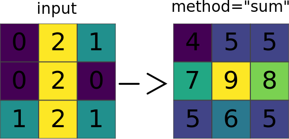
r.neighbors looks at each cell in a raster input map, and examines the values assigned to the cells in some user-defined "neighborhood" around it. It outputs a new raster map layer in which each cell is assigned a value that is some (user-specified) function of the values in that cell's neighborhood. For example, each cell in the output layer might be assigned a value equal to the average of the values appearing in its 3 x 3 cell "neighborhood" in the input layer. Note that the centre cell is also included in the calculation.
Figure: Illustration for an 3x3 average neighborhood
OPTIONS
The user must specify the names of the raster map layers to be used for input and output, the method used to analyze neighborhood values (i.e., the neighborhood function or operation to be performed), and the size of the neighborhood.The user can optionally specify a selection map, to compute new values only where the raster cells of the selection map are not NULL. In case of a NULL cells, the values from the input map are copied into the output map. This may useful to smooth only parts of an elevation map (pits, peaks, ...).
Example how to use a selection map with method=average:
input map:
1 1  1 1 1
1 1  1 1 1
1 1 10 1 1
1 1  1 1 1
1 1  1 1 1
* * * * *
* * 1 * *
* 1 1 1 *
* * 1 * *
* * * * *
1 1 1 1 1
1 1 2 1 1
1 2 2 2 1
1 1 2 1 1
1 1 1 1 1
1 1 1 1 1
1 2 2 2 1
1 2 2 2 1
1 2 2 2 1
1 1 1 1 1
It is also possible to weigh cells within the neighborhood. This can be either done with a custom weights matrix or by specifying a weighting function.
In order to use a custom weights matrix, file needs to be specified as a weighting_function and a path to a text file containing the weights needs to be given in the weight option.
Alternatively, gaussian and exponential weighting functions can be selected as weighting function.
For the gaussian weighting function, the user specifies the sigma value (σ) for the gauss filter in the weighting_factor option. The sigma value represents the standard deviation of the gaussian distribution, where the weighting formula for the gaussian filter is defined as follows:
exp(-(x*x+y*y)/(2*σ^2))/(2*π*σ^2)
Lower values for sigma result in a steeper curve, so that more weight is put on cells close to the center of the moving window with a steeper decrease in weights with distance from the center.
For the exponential weighting function, the user specifies a factor for an exponential kernel in the weighting_factor. Negative factors result in negative exponential decrease in weights from the center cell. The weighting formula for the exponential kernel is defined as follows:
exp(factor*sqrt(x*x+y*y))
Stronger negative values for the factor result in a steeper curve, so that more weight is put on cells close to the center of the moving window with a steeper decrease in weights with distance from the center.
Optionally, the user can also run r.neighbors specify the TITLE to be assigned to the raster map layer output, select to not align the resolution of the output with that of the input (the -a option). These options are described further below.
Neighborhood Operation Methods: The neighborhood operators determine what new value a center cell in a neighborhood will have after examining values inside its neighboring cells. Each cell in a raster map layer becomes the center cell of a neighborhood as the neighborhood window moves from cell to cell throughout the map layer. r.neighbors can perform the following operations:
- average
- The average value within the neighborhood.
In the following example, the result would be:
(7*4 + 6 + 5 + 4*3)/9 = 5.6667
The result is rounded to the nearest integer (in this case 6).Raw Data Operation New Data +---+---+---+ +---+---+---+ | 7 | 7 | 5 | | | | | +---+---+---+ average +---+---+---+ | 4 | 7 | 4 |--------->| | 6 | | +---+---+---+ +---+---+---+ | 7 | 6 | 4 | | | | | +---+---+---+ +---+---+---+
- median
- The value found half-way through a list of the neighborhood's values, when these are ranged in numerical order.
- mode
- The most frequently occurring value in the neighborhood.
- minimum
- The minimum value within the neighborhood.
- maximum
- The maximum value within the neighborhood.
- range
- The range value within the neighborhood.
- stddev
- The statistical standard deviation of values within the neighborhood (rounded to the nearest integer).
- sum
- The sum of values within the neighborhood.
- count
- The count of filled (not NULL) cells.
- variance
- The statistical variance of values within the neighborhood (rounded to the nearest integer).
- diversity
- The number of different values within the neighborhood. In the above example, the diversity is 4.
- interspersion
- The percentage of cells containing values which differ from the values
assigned to the center cell in the neighborhood, plus 1.
In the above example, the interspersion is:
5/8 * 100 + 1 = 63.5
The result is rounded to the nearest integer (in this case 64). - quart1, quart3
- The result will be the first or the third quartile (equal of 25th and 75th percentiles).
- perc90
- The result will be the 90th percentile of neighborhood.
- quantile
- Any quantile as specified by "quantile" input parameter.
Neighborhood Size:
The neighborhood size specifies which cells surrounding any given
cell fall into the neighborhood for that cell.
The size must be an odd integer and represent the length of one of
moving window edges in cells.
For example, a size value of 3 will result in
                              _ _ _
                             |_|_|_|
    3 x 3 neighborhood --->  |_|_|_|
                             |_|_|_|
Matrix weights: A custom matrix can be used if none of the neighborhood operation methods are desirable by using the weight. This option must be used in conjunction with the size option to specify the matrix size and file needs to be specified as weighting_function. The weights desired are to be entered into a text file. For example, to calculate the focal mean with a matrix size of 3,
r.neigbors in=input.map out=output.map size=3 weighting_function=file \
weight=weights.txt
3 3 3
1 4 8
9 5 3
+-+-+-+
|3|3|3|
+-+-+-+
|1|4|8|
+-+-+-+
|9|5|3|
+-+-+-+
 0 1 1 1 0
 1 0 0 0 1
 1 0 0 0 1
 1 0 0 0 1
 0 1 1 1 0
sum(w[i]*x[i]) / sum(w[i])
FLAGS
- -a
- If specified, r.neighbors will not align the output
raster map layer with that of the input raster map layer.
The r.neighbors program works in the current geographic region.
It is recommended, but not required, that the resolution
of the geographic region be the same as that of the raster map layer.
By default, if unspecified,
r.neighbors will align these geographic region settings.
- -c
-
This flag will use a circular neighborhood for the moving analysis window,
centered on the current cell.
The exact masks for the first few neighborhood sizes are as follows:
3x3     . X .        5x5    . . X . .    7x7    . . . X . . .
        X O X               . X X X .           . X X X X X .
        . X .               X X O X X           . X X X X X .
                            . X X X .           X X X O X X X
                            . . X . .           . X X X X X .
                                                . X X X X X .
                                                . . . X . . .


9x9    . . . . X . . . .        11x11   . . . . . X . . . . .
       . . X X X X X . .                . . X X X X X X X . .
       . X X X X X X X .                . X X X X X X X X X .
       . X X X X X X X .                . X X X X X X X X X .
       X X X X O X X X X                . X X X X X X X X X .
       . X X X X X X X .                X X X X X O X X X X X
       . X X X X X X X .                . X X X X X X X X X .
       . . X X X X X . .                . X X X X X X X X X .
       . . . . X . . . .                . X X X X X X X X X .
                                        . . X X X X X X X . .
                                        . . . . . X . . . . .
NOTES
The r.neighbors program works in the current geographic region with the current mask, if any. It is recommended, but not required, that the resolution of the geographic region be the same as that of the raster map layer. By default, r.neighbors will align these geographic region settings. However, the user can select to keep original input and output resolutions which are not aligned by specifying this (e.g., using the -a option).r.neighbors doesn't propagate NULLs, but computes the aggregate over the non-NULL cells in the neighborhood.
The -c flag and the weights parameter are mutually exclusive. Any use of the two together will produce an error. Differently-shaped neighborhood analysis windows may be achieved by using the weight= parameter to specify a weights file where all values are equal. The user can also vary the weights at the edge of the neighborhood according to the proportion of the cell that lies inside the neighborhood circle, effectively anti-aliasing the analysis mask.
For aggregates where a weighted calculation isn't meaningful (specifically: minimum, maximum, diversity and interspersion), the weights are used to create a binary mask, where zero causes the cell to be ignored and any non-zero value causes the cell to be used.
r.neighbors copies the GRASS color files associated with the input raster map layer for those output map layers that are based on the neighborhood average, median, mode, minimum, and maximum. Because standard deviation, variance, diversity, and interspersion are indices, rather than direct correspondents to input values, no color files are copied for these map layers. (The user should note that although the color file is copied for average neighborhood function output, whether or not the color file makes sense for the output will be dependent on the input data values.)
Propagation of output precision
The following logic has been implemented: For any aggregate, there are two factors affecting the output type:- Whether the input map is integer or floating-point.
- Whether the weighted or unweighted version of the aggregate is used.
| input type/weight | integer | float | ||
|---|---|---|---|---|
| no | yes | no | yes | |
| average | float | float | float | float |
| median | [1] | [1] | float | float |
| mode | integer | integer | [2] | [2] |
| minimum | integer | integer | float | float |
| maximum | integer | integer | float | float |
| range | integer | integer | float | float |
| stddev | float | float | float | float |
| sum | integer | float | float | float |
| count | integer | float | integer | float |
| variance | float | float | float | float |
| diversity | integer | integer | integer | integer |
| interspersion | integer | integer | integer | integer |
| quart1 | [1] | [1] | float | float |
| quart3 | [1] | [1] | float | float |
| perc90 | [1] | [1] | float | float |
| quantile | [1] | [1] | float | float |
[1] For integer input, quantiles may produce float results from
interpolating between adjacent values.
[2] Calculating the mode of floating-point data is essentially
meaningless.
With the current aggregates, there are 5 cases:
- Output is always float: average, variance, stddev, quantiles (with interpolation).
- Output is always integer: diversity, interspersion.
- Output is integer if unweighted, float if weighted: count.
- Output matches input: minimum, maximum, range, mode (subject to note 2 above), quantiles (without interpolation).
- Output is integer for integer input and unweighted aggregate, otherwise float: sum.
Performance
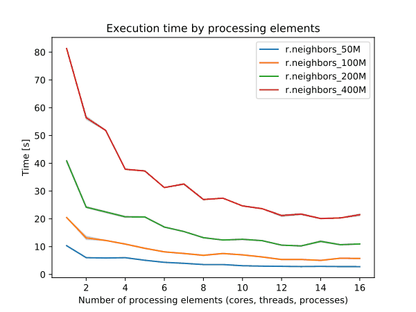
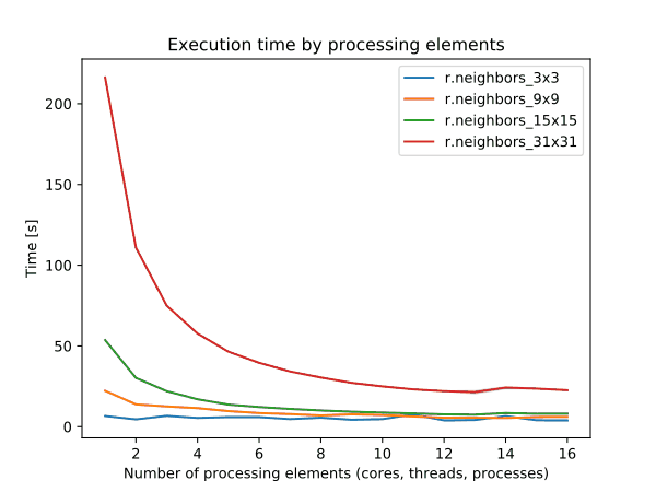
To enable parallel processing, the user can specify the number of threads to be used with the nprocs parameter (default 1). The memory parameter (default 300) can also be provided to determine the size of the buffer for computation.


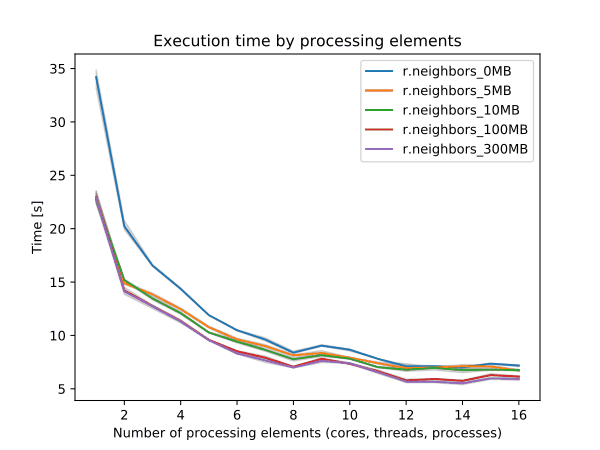
Figure: Benchmark on the left shows execution time for different number of cells, benchmark in the middle shows execution time for different sizes of neighborhood for a 10000x10000 raster and benchmark on the right shows execution time for different memory size for a 10000x10000 raster. See benchmark scripts in source code. (Intel Core i9-10940X CPU @ 3.30GHz x 28)
To reduce the memory requirements to minimum, set option memory to zero. To take advantage of the parallelization, GRASS GIS needs to be compiled with OpenMP enabled.
EXAMPLES
Measure occupancy of neighborhood
Set up 10x10 computational region to aid visual inspection of resultsg.region rows=10 cols=10
r.random.cells output=random_cells distance=0 ncells=50
r.neighbors input=random_cells output=counts method=count
r.mapcalc "count_around = if( isnull(random_cells), counts, counts - 1)"
SEE ALSO
g.region, r.clump, r.mapcalc, r.mfilter, r.statistics, r.supportAUTHORS
Original version: Michael Shapiro, U.S.Army Construction Engineering Research LaboratoryUpdates for GRASS GIS 7 by Glynn Clements and others
SOURCE CODE
Available at: r.neighbors source code (history)
Accessed: Monday Feb 24 17:50:42 2025
Main index | Raster index | Topics index | Keywords index | Graphical index | Full index
© 2003-2025 GRASS Development Team, GRASS GIS 8.4.1 Reference Manual