TransverseMercator and TransverseMercatorExact provide accurate implementations of the transverse Mercator projection. The TransverseMercatorProj utility provides an interface to these classes.
Go to
- Test data for the transverse Mercator projection
- Series approximation for transverse Mercator
- Figures from paper on transverse Mercator projection
References:
- L. Krüger, Konforme Abbildung des Erdellipsoids in der Ebene (Conformal mapping of the ellipsoidal earth to the plane), Royal Prussian Geodetic Institute, New Series 52, 172 pp. (1912).
- L. P. Lee, Conformal Projections Based on Elliptic Functions, (B. V. Gutsell, Toronto, 1976), 128pp., ISBN: 0919870163 (Also appeared as: Monograph 16, Suppl. No. 1 to Canadian Cartographer, Vol 13). Part V, pp. 67–101, Conformal Projections Based On Jacobian Elliptic Functions; borrow from archive.org.
- C. F. F. Karney, Transverse Mercator with an accuracy of a few nanometers, J. Geodesy 85(8), 475–485 (Aug. 2011); addenda: tm-addenda.html; preprint: arXiv:1002.1417; resource page: tm.html.
The algorithm for TransverseMercator is based on Krüger (1912); that for TransverseMercatorExact is based on Lee (1976).
See tm-grid.kmz, for an illustration of the exact transverse Mercator grid in Google Earth.
Test data for the transverse Mercator projection
A test set for the transverse Mercator projection is available at
- TMcoords.dat.gz
- C. F. F. Karney, Test data for the transverse Mercator projection (2009),
DOI: 10.5281/zenodo.32470.
This is about 17 MB (compressed). This test set consists of a set of geographic coordinates together with the corresponding transverse Mercator coordinates. The WGS84 ellipsoid is used, with central meridian 0°, central scale factor 0.9996 (the UTM value), false easting = false northing = 0 m.
Each line of the test set gives 6 space delimited numbers
- latitude (degrees, exact)
- longitude (degrees, exact — see below)
- easting (meters, accurate to 0.1 pm)
- northing (meters, accurate to 0.1 pm)
- meridian convergence (degrees, accurate to 10−18 deg)
- scale (accurate to 10−20)
The latitude and longitude are all multiples of 10−12 deg and should be regarded as exact, except that longitude = 82.63627282416406551 should be interpreted as exactly (1 − e) 90°. These results are computed using Lee's formulas with Maxima's bfloats and fpprec set to 80 (so the errors in the data are probably 1/2 of the values quoted above). The Maxima code, tm.mac and ellint.mac, was used to prepare this data set is included in the distribution; you will need to have Maxima installed to use this code. The comments at the top of tm.mac illustrate how to run it.
The contents of the file are as follows:
- 250000 entries randomly distributed in lat in [0°, 90°], lon in [0°, 90°];
- 1000 entries randomly distributed on lat in [0°, 90°], lon = 0°;
- 1000 entries randomly distributed on lat = 0°, lon in [0°, 90°];
- 1000 entries randomly distributed on lat in [0°, 90°], lon = 90°;
- 1000 entries close to lat = 90° with lon in [0°, 90°];
- 1000 entries close to lat = 0°, lon = 0° with lat ≥ 0°, lon ≥ 0°;
- 1000 entries close to lat = 0°, lon = 90° with lat ≥ 0°, lon ≤ 90°;
- 2000 entries close to lat = 0°, lon = (1 − e) 90° with lat ≥ 0°;
- 25000 entries randomly distributed in lat in [−89°, 0°], lon in [(1 − e) 90°, 90°];
- 1000 entries randomly distributed on lat in [−89°, 0°], lon = 90°;
- 1000 entries randomly distributed on lat in [−89°, 0°], lon = (1 − e) 90°;
- 1000 entries close to lat = 0°, lon = 90° (lat < 0°, lon ≤ 90°);
- 1000 entries close to lat = 0°, lon = (1 − e) 90° (lat < 0°, lon ≤ (1 − e) 90°);
(a total of 287000 entries). The entries for lat < 0° and lon in [(1 − e) 90°, 90°] use the "extended" domain for the transverse Mercator projection explained in Sec. 5 of Karney (2011). The first 258000 entries have lat ≥ 0° and are suitable for testing implementations following the standard convention.
Series approximation for transverse Mercator
Krüger (1912) gives a 4th-order approximation to the transverse Mercator projection. This is accurate to about 200 nm (200 nanometers) within the UTM domain. Here we present the series extended to 10th order. By default, TransverseMercator uses the 6th-order approximation. The preprocessor macro GEOGRAPHICLIB_TRANSVERSEMERCATOR_ORDER can be used to select an order from 4 thru 8. The series expanded to order n30 are given in tmseries30.html.
In the formulas below ^ indicates exponentiation (n^3 = n*n*n) and / indicates real division (3/5 = 0.6). The equations need to be converted to Horner form, but are here left in expanded form so that they can be easily truncated to lower order in n. Some of the integers here are not representable as 32-bit integers and will need to be included as 64-bit integers.
A in Krüger, p. 12, eq. (5)
  A = a/(n + 1) * (1 + 1/4 * n^2
                     + 1/64 * n^4
                     + 1/256 * n^6
                     + 25/16384 * n^8
                     + 49/65536 * n^10);
γ in Krüger, p. 21, eq. (41)
alpha[1] =   1/2 * n
           - 2/3 * n^2
           + 5/16 * n^3
           + 41/180 * n^4
           - 127/288 * n^5
           + 7891/37800 * n^6
           + 72161/387072 * n^7
           - 18975107/50803200 * n^8
           + 60193001/290304000 * n^9
           + 134592031/1026432000 * n^10;
alpha[2] =   13/48 * n^2
           - 3/5 * n^3
           + 557/1440 * n^4
           + 281/630 * n^5
           - 1983433/1935360 * n^6
           + 13769/28800 * n^7
           + 148003883/174182400 * n^8
           - 705286231/465696000 * n^9
           + 1703267974087/3218890752000 * n^10;
alpha[3] =   61/240 * n^3
           - 103/140 * n^4
           + 15061/26880 * n^5
           + 167603/181440 * n^6
           - 67102379/29030400 * n^7
           + 79682431/79833600 * n^8
           + 6304945039/2128896000 * n^9
           - 6601904925257/1307674368000 * n^10;
alpha[4] =   49561/161280 * n^4
           - 179/168 * n^5
           + 6601661/7257600 * n^6
           + 97445/49896 * n^7
           - 40176129013/7664025600 * n^8
           + 138471097/66528000 * n^9
           + 48087451385201/5230697472000 * n^10;
alpha[5] =   34729/80640 * n^5
           - 3418889/1995840 * n^6
           + 14644087/9123840 * n^7
           + 2605413599/622702080 * n^8
           - 31015475399/2583060480 * n^9
           + 5820486440369/1307674368000 * n^10;
alpha[6] =   212378941/319334400 * n^6
           - 30705481/10378368 * n^7
           + 175214326799/58118860800 * n^8
           + 870492877/96096000 * n^9
           - 1328004581729009/47823519744000 * n^10;
alpha[7] =   1522256789/1383782400 * n^7
           - 16759934899/3113510400 * n^8
           + 1315149374443/221405184000 * n^9
           + 71809987837451/3629463552000 * n^10;
alpha[8] =   1424729850961/743921418240 * n^8
           - 256783708069/25204608000 * n^9
           + 2468749292989891/203249958912000 * n^10;
alpha[9] =   21091646195357/6080126976000 * n^9
           - 67196182138355857/3379030566912000 * n^10;
alpha[10]=   77911515623232821/12014330904576000 * n^10;
β in Krüger, p. 18, eq. (26*)
 beta[1] =   1/2 * n
           - 2/3 * n^2
           + 37/96 * n^3
           - 1/360 * n^4
           - 81/512 * n^5
           + 96199/604800 * n^6
           - 5406467/38707200 * n^7
           + 7944359/67737600 * n^8
           - 7378753979/97542144000 * n^9
           + 25123531261/804722688000 * n^10;
 beta[2] =   1/48 * n^2
           + 1/15 * n^3
           - 437/1440 * n^4
           + 46/105 * n^5
           - 1118711/3870720 * n^6
           + 51841/1209600 * n^7
           + 24749483/348364800 * n^8
           - 115295683/1397088000 * n^9
           + 5487737251099/51502252032000 * n^10;
 beta[3] =   17/480 * n^3
           - 37/840 * n^4
           - 209/4480 * n^5
           + 5569/90720 * n^6
           + 9261899/58060800 * n^7
           - 6457463/17740800 * n^8
           + 2473691167/9289728000 * n^9
           - 852549456029/20922789888000 * n^10;
 beta[4] =   4397/161280 * n^4
           - 11/504 * n^5
           - 830251/7257600 * n^6
           + 466511/2494800 * n^7
           + 324154477/7664025600 * n^8
           - 937932223/3891888000 * n^9
           - 89112264211/5230697472000 * n^10;
 beta[5] =   4583/161280 * n^5
           - 108847/3991680 * n^6
           - 8005831/63866880 * n^7
           + 22894433/124540416 * n^8
           + 112731569449/557941063680 * n^9
           - 5391039814733/10461394944000 * n^10;
 beta[6] =   20648693/638668800 * n^6
           - 16363163/518918400 * n^7
           - 2204645983/12915302400 * n^8
           + 4543317553/18162144000 * n^9
           + 54894890298749/167382319104000 * n^10;
 beta[7] =   219941297/5535129600 * n^7
           - 497323811/12454041600 * n^8
           - 79431132943/332107776000 * n^9
           + 4346429528407/12703122432000 * n^10;
 beta[8] =   191773887257/3719607091200 * n^8
           - 17822319343/336825216000 * n^9
           - 497155444501631/1422749712384000 * n^10;
 beta[9] =   11025641854267/158083301376000 * n^9
           - 492293158444691/6758061133824000 * n^10;
 beta[10]=   7028504530429621/72085985427456000 * n^10;
The high-order expansions for α and β were produced by the Maxima program tmseries.mac (included in the distribution). To run, start Maxima and enter
load("tmseries.mac")$
Further instructions are included at the top of the file.
Figures from paper on transverse Mercator projection
This section gives color versions of the figures in
- C. F. F. Karney, Transverse Mercator with an accuracy of a few nanometers, J. Geodesy 85(8), 475–485 (Aug. 2011); addenda: tm-addenda.html; preprint: arXiv:1002.1417; resource page: tm.html.
NOTE: The numbering of the figures matches that in the paper cited above. The figures in this section are relatively small in order to allow them to be displayed quickly. Vector versions of these figures are available in tm-figs.pdf. This allows you to magnify the figures to show the details more clearly.
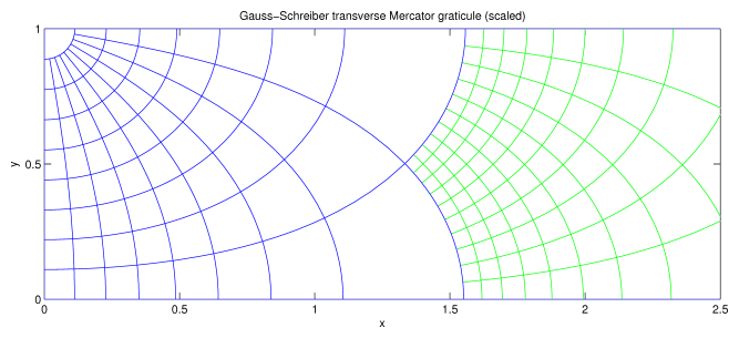
Fig. 1(a): The graticule for the spherical transverse Mercator projection. The equator lies on y = 0. Compare this with Lee, Fig. 1 (right), which shows the graticule for half a sphere, but note that in his notation x and y have switched meanings. The graticule for the ellipsoid differs from that for a sphere only in that the latitude lines have shifted slightly. (The conformal transformation from an ellipsoid to a sphere merely relabels the lines of latitude.) This projection places the point latitude = 0°, longitude = 90° at infinity.
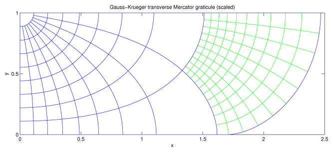
Fig. 1(b): The graticule for the Gauss-Krüger transverse Mercator projection. The equator lies on y = 0 for longitude < 81°; beyond this, it arcs up to meet y = 1. Compare this with Lee, Fig. 45 (upper), which shows the graticule for the International Ellipsoid. Lee, Fig. 46, shows the graticule for the entire ellipsoid. This projection (like the Thompson projection) projects the ellipsoid to a finite area.
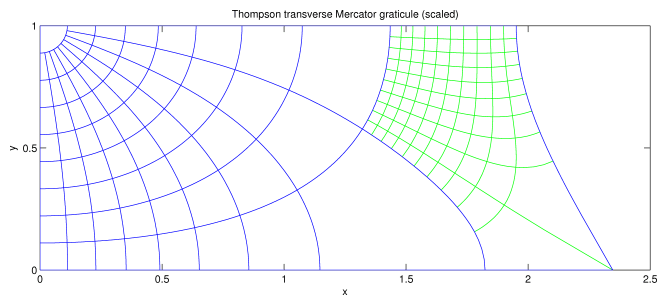
Fig. 1(c): The graticule for the Thompson transverse Mercator projection. The equator lies on y = 0 for longitude < 81°; at longitude = 81°, it turns by 120° and heads for y = 1. Compare this with Lee, Fig. 43, which shows the graticule for the International Ellipsoid. Lee, Fig. 44, shows the graticule for the entire ellipsoid. This projection (like the Gauss-Krüger projection) projects the ellipsoid to a finite area.
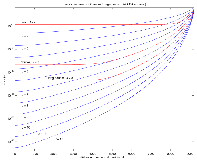
Fig. 2: The truncation error for the series for the Gauss-Krüger transverse Mercator projection. The blue curves show the truncation error for the order of the series J = 2 (top) thru J = 12 (bottom). The red curves show the combined truncation and round-off errors for
- float and J = 4 (top)
- double and J = 6 (middle)
- long double and J = 8 (bottom)
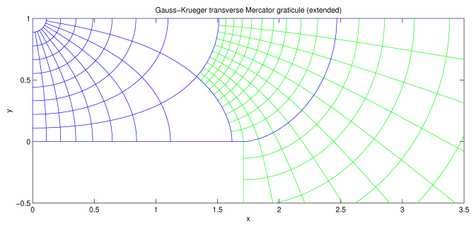
Fig. 3(a): The graticule for the extended domain. The blue lines show latitude and longitude at multiples of 10°. The green lines show 1° intervals for longitude in [80°, 90°] and latitude in [−5°, 10°].
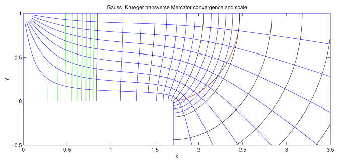
Fig. 3(b): The convergence and scale for the Gauss-Krüger transverse Mercator projection in the extended domain. The blue lines emanating from the top left corner (the north pole) are lines of constant convergence. Convergence = 0° is given by the dog-legged line joining the points (0,1), (0,0), (1.71,0), (1.71,−∞). Convergence = 90° is given by the line y = 1. The other lines show multiples of 10° between 0° and 90°. The other blue, the green and the black lines show scale = 1 thru 2 at intervals of 0.1, 2 thru 15 at intervals of 1, and 15 thru 35 at intervals of 5. Multiples of 5 are shown in black, multiples of 1 are shown in blue, and the rest are shown in green. Scale = 1 is given by the line segment (0,0) to (0,1). The red line shows the equator between lon = 81° and 90°. The scale and convergence at the branch point are 1/e = 10 and 0°, respectively.

Fig. 3(c): The graticule for the Thompson transverse Mercator projection for the extended domain. The range of the projection is the rectangular region shown
- 0 ≤ u ≤ K(e2), 0 ≤ v ≤ K(1 − e2)
The coloring of the lines is the same as Fig. 3(a), except that latitude lines extended down to −10° and a red line has been added showing the line y = 0 for x > 1.71 in the Gauss-Krüger projection (Fig. 3(a)). The extended Thompson projection figure has reflection symmetry on all the four sides of Fig. 3(c).