Geodesic and GeodesicLine provide accurate solutions to the direct and inverse geodesic problems. The GeodSolve utility provides an interface to these classes. AzimuthalEquidistant implements the azimuthal equidistant projection in terms of geodesics. CassiniSoldner implements a transverse cylindrical equidistant projection in terms of geodesics. The GeodesicProj utility provides an interface to these projections.
The algorithms used by Geodesic and GeodesicLine are based on a Taylor expansion of the geodesic integrals valid when the flattening f is small. GeodesicExact and GeodesicLineExact evaluate the integrals exactly (in terms of incomplete elliptic integrals). For the WGS84 ellipsoid, the series solutions are about 2–3 times faster and 2–3 times more accurate (because it's easier to control round-off errors with series solutions); thus Geodesic and GeodesicLine are recommended for most geodetic applications. However, in applications where the absolute value of f is greater than about 0.02, the exact classes should be used.
Go to
- Test data for geodesics
- Expansions for geodesics
- Geodesics in terms of elliptic integrals
- Parameters for the meridian
- Short geodesics
For some background information on geodesics on triaxial ellipsoids, see Geodesics on a triaxial ellipsoid.
References:
- F. W. Bessel, The calculation of longitude and latitude from geodesic measurements (1825), Astron. Nachr. 331(8), 852–861 (2010); translated by C. F. F. Karney and R. E. Deakin; preprint: arXiv:0908.1824.
- F. R. Helmert, Mathematical and Physical Theories of Higher Geodesy, Part 1 (1880), Aeronautical Chart and Information Center (St. Louis, 1964), Chaps. 5–7.
- J. Danielsen, The area under the geodesic, Survey Review 30(232), 61–66 (1989). DOI: 10.1179/003962689791474267
- C. F. F. Karney, Algorithms for geodesics, J. Geodesy 87(1), 43–55 (2013); DOI: 10.1007/s00190-012-0578-z; addenda: geod-addenda.html; resource page: geod.html.
- A collection of some papers on geodesics is available at https://geographiclib.sourceforge.io/geodesic-papers/biblio.html
- The wikipedia page, Geodesics on an ellipsoid.
Test data for geodesics
A test set a geodesics is available at
- GeodTest.dat.gz
- C. F. F. Karney, Test set for geodesics (2010),
DOI: 10.5281/zenodo.32156.
This is about 39 MB (compressed). This consists of a set of geodesics for the WGS84 ellipsoid. A subset of this (consisting of 1/50 of the members — about 690 kB, compressed) is available at
Each line of the test set gives 10 space delimited numbers
- latitude at point 1, lat1 (degrees, exact)
- longitude at point 1, lon1 (degrees, always 0)
- azimuth at point 1, azi1 (clockwise from north in degrees, exact)
- latitude at point 2, lat2 (degrees, accurate to 10−18 deg)
- longitude at point 2, lon2 (degrees, accurate to 10−18 deg)
- azimuth at point 2, azi2 (degrees, accurate to 10−18 deg)
- geodesic distance from point 1 to point 2, s12 (meters, exact)
- arc distance on the auxiliary sphere, a12 (degrees, accurate to 10−18 deg)
- reduced length of the geodesic, m12 (meters, accurate to 0.1 pm)
- the area under the geodesic, S12 (m2, accurate to 1 mm2)
These are computed using as direct geodesic calculations with the given lat1, lon1, azi1, and s12. The distance s12 always corresponds to an arc length a12 ≤ 180°, so the given geodesics give the shortest paths from point 1 to point 2. For simplicity and without loss of generality, lat1 is chosen in [0°, 90°], lon1 is taken to be zero, azi1 is chosen in [0°, 180°]. Furthermore, lat1 and azi1 are taken to be multiples of 10−12 deg and s12 is a multiple of 0.1 μm in [0 m, 20003931.4586254 m]. This results in lon2 in [0°, 180°] and azi2 in [0°, 180°].
The direct calculation uses an expansion of the geodesic equations accurate to f30 (approximately 1 part in 1050) and is computed with with Maxima's bfloats and fpprec set to 100 (so the errors in the data are probably 1/2 of the values quoted above).
The contents of the file are as follows:
- 100000 entries randomly distributed
- 50000 entries which are nearly antipodal
- 50000 entries with short distances
- 50000 entries with one end near a pole
- 50000 entries with both ends near opposite poles
- 50000 entries which are nearly meridional
- 50000 entries which are nearly equatorial
- 50000 entries running between vertices (azi1 = azi2 = 90°)
- 50000 entries ending close to vertices
(a total of 500000 entries). The values for s12 for the geodesics running between vertices are truncated to a multiple of 0.1 pm and this is used to determine point 2.
This data can be fed to the GeodSolve utility as follows
- Direct from point 1:
gunzip -c GeodTest.dat.gz | cut -d' ' -f1,2,3,7 | ./GeodSolve
This should yield columns 4, 5, 6, and 9 of the test set. - Direct from point 2:
gunzip -c GeodTest.dat.gz | cut -d' ' -f4,5,6,7 | sed "s/ \([^ ]*$\)/ -\1/" | ./GeodSolve
(The sed command negates the distance.) This should yield columns 1, 2, and 3, and the negative of column 9 of the test set. - Inverse between points 1 and 2:
gunzip -c GeodTest.dat.gz | cut -d' ' -f1,2,4,5 | ./GeodSolve -i
This should yield columns 3, 6, 7, and 9 of the test set.
Add, e.g., "-p 6", to the call to GeodSolve to change the precision of the output. Adding "-f" causes GeodSolve to print 12 fields specifying the geodesic; these include the 10 fields in the test set plus the geodesic scales M12 and M21 which are inserted between m12 and S12.
Code for computing arbitrarily accurate geodesics in maxima is available in geodesic.mac (this depends on ellint.mac and uses the series computed by geod.mac). This solve both the direct and inverse geodesic problems and offers the ability to solve the problems either using series expansions (similar to Geodesic) or in terms of elliptic integrals (similar to GeodesicExact).
Expansions for geodesics
We give here the series expansions for the various geodesic integrals valid to order f10. In this release of the code, we use a 6th-order expansions. This is sufficient to maintain accuracy for doubles for the SRMmax ellipsoid (a = 6400 km, f = 1/150). However, the preprocessor macro GEOGRAPHICLIB_GEODESIC_ORDER can be used to select an order from 3 thru 8. (If using long doubles, with a 64-bit fraction, the default order is 7.) The series expanded to order f30 are given in geodseries30.html.
In the formulas below ^ indicates exponentiation (f^3 = f3) and / indicates real division (3/5 = 0.6). The equations need to be converted to Horner form, but are here left in expanded form so that they can be easily truncated to lower order. These expansions were obtained using the Maxima code, geod.mac.
In the expansions below, we have
- \( \alpha \) is the azimuth
- \( \alpha_0 \) is the azimuth at the equator crossing
- \( \lambda \) is the longitude measured from the equator crossing
- \( \sigma \) is the spherical arc length
- \( \omega = \tan^{-1}(\sin\alpha_0\tan\sigma) \) is the spherical longitude
- \( a \) is the equatorial radius
- \( b \) is the polar semi-axis
- \( f \) is the flattening
- \( e^2 = f(2 - f) \)
- \( e'^2 = e^2/(1-e^2) \)
- \( k^2 = e'^2 \cos^2\alpha_0 = 4 \epsilon / (1 - \epsilon)^2 \)
- \( n = f / (2 - f) \)
- \( c^2 = a^2/2 + b^2/2 (\tanh^{-1}e)/e \)
- ep2 = \( e'^2 \)
- k2 = \( k^2 \)
- eps = \( \epsilon = k^2 / (\sqrt{1 + k^2} + 1)^2\)
The formula for distance is
\[ \frac sb = I_1(\sigma) \]
where
\[ \begin{align} I_1(\sigma) &= A_1\bigl(\sigma + B_1(\sigma)\bigr) \\ B_1(\sigma) &= \sum_{j=1} C_{1j} \sin 2j\sigma \end{align} \]
and
A1 = (1 + 1/4 * eps^2
        + 1/64 * eps^4
        + 1/256 * eps^6
        + 25/16384 * eps^8
        + 49/65536 * eps^10) / (1 - eps);
C1[1] = - 1/2 * eps
        + 3/16 * eps^3
        - 1/32 * eps^5
        + 19/2048 * eps^7
        - 3/4096 * eps^9;
C1[2] = - 1/16 * eps^2
        + 1/32 * eps^4
        - 9/2048 * eps^6
        + 7/4096 * eps^8
        + 1/65536 * eps^10;
C1[3] = - 1/48 * eps^3
        + 3/256 * eps^5
        - 3/2048 * eps^7
        + 17/24576 * eps^9;
C1[4] = - 5/512 * eps^4
        + 3/512 * eps^6
        - 11/16384 * eps^8
        + 3/8192 * eps^10;
C1[5] = - 7/1280 * eps^5
        + 7/2048 * eps^7
        - 3/8192 * eps^9;
C1[6] = - 7/2048 * eps^6
        + 9/4096 * eps^8
        - 117/524288 * eps^10;
C1[7] = - 33/14336 * eps^7
        + 99/65536 * eps^9;
C1[8] = - 429/262144 * eps^8
        + 143/131072 * eps^10;
C1[9] = - 715/589824 * eps^9;
C1[10] = - 2431/2621440 * eps^10;
The function \( \tau(\sigma) = s/(b A_1) = \sigma + B_1(\sigma) \) may be inverted by series reversion giving
\[ \sigma(\tau) = \tau + \sum_{j=1} C'_{1j} \sin 2j\sigma \]
where
C1'[1] = + 1/2 * eps
         - 9/32 * eps^3
         + 205/1536 * eps^5
         - 4879/73728 * eps^7
         + 9039/327680 * eps^9;
C1'[2] = + 5/16 * eps^2
         - 37/96 * eps^4
         + 1335/4096 * eps^6
         - 86171/368640 * eps^8
         + 4119073/28311552 * eps^10;
C1'[3] = + 29/96 * eps^3
         - 75/128 * eps^5
         + 2901/4096 * eps^7
         - 443327/655360 * eps^9;
C1'[4] = + 539/1536 * eps^4
         - 2391/2560 * eps^6
         + 1082857/737280 * eps^8
         - 2722891/1548288 * eps^10;
C1'[5] = + 3467/7680 * eps^5
         - 28223/18432 * eps^7
         + 1361343/458752 * eps^9;
C1'[6] = + 38081/61440 * eps^6
         - 733437/286720 * eps^8
         + 10820079/1835008 * eps^10;
C1'[7] = + 459485/516096 * eps^7
         - 709743/163840 * eps^9;
C1'[8] = + 109167851/82575360 * eps^8
         - 550835669/74317824 * eps^10;
C1'[9] = + 83141299/41287680 * eps^9;
C1'[10] = + 9303339907/2972712960 * eps^10;
The reduced length is given by
\[ \begin{align} \frac mb &= \sqrt{1 + k^2 \sin^2\sigma_2} \cos\sigma_1 \sin\sigma_2 \\ &\quad {}-\sqrt{1 + k^2 \sin^2\sigma_1} \sin\sigma_1 \cos\sigma_2 \\ &\quad {}-\cos\sigma_1 \cos\sigma_2 \bigl(J(\sigma_2) - J(\sigma_1)\bigr) \end{align} \]
where
\[ \begin{align} J(\sigma) &= I_1(\sigma) - I_2(\sigma) \\ I_2(\sigma) &= A_2\bigl(\sigma + B_2(\sigma)\bigr) \\ B_2(\sigma) &= \sum_{j=1} C_{2j} \sin 2j\sigma \end{align} \]
A2 = (1 - 3/4 * eps^2
        - 7/64 * eps^4
        - 11/256 * eps^6
        - 375/16384 * eps^8
        - 931/65536 * eps^10) / (1 + eps);
C2[1] = + 1/2 * eps
        + 1/16 * eps^3
        + 1/32 * eps^5
        + 41/2048 * eps^7
        + 59/4096 * eps^9;
C2[2] = + 3/16 * eps^2
        + 1/32 * eps^4
        + 35/2048 * eps^6
        + 47/4096 * eps^8
        + 557/65536 * eps^10;
C2[3] = + 5/48 * eps^3
        + 5/256 * eps^5
        + 23/2048 * eps^7
        + 191/24576 * eps^9;
C2[4] = + 35/512 * eps^4
        + 7/512 * eps^6
        + 133/16384 * eps^8
        + 47/8192 * eps^10;
C2[5] = + 63/1280 * eps^5
        + 21/2048 * eps^7
        + 51/8192 * eps^9;
C2[6] = + 77/2048 * eps^6
        + 33/4096 * eps^8
        + 2607/524288 * eps^10;
C2[7] = + 429/14336 * eps^7
        + 429/65536 * eps^9;
C2[8] = + 6435/262144 * eps^8
        + 715/131072 * eps^10;
C2[9] = + 12155/589824 * eps^9;
C2[10] = + 46189/2621440 * eps^10;
The longitude is given in terms of the spherical longitude by
\[ \lambda = \omega - f \sin\alpha_0 I_3(\sigma) \]
where
\[ \begin{align} I_3(\sigma) &= A_3\bigl(\sigma + B_3(\sigma)\bigr) \\ B_3(\sigma) &= \sum_{j=1} C_{3j} \sin 2j\sigma \end{align} \]
and
A3 = 1 - (1/2 - 1/2*n) * eps
       - (1/4 + 1/8*n - 3/8*n^2) * eps^2
       - (1/16 + 3/16*n + 1/16*n^2 - 5/16*n^3) * eps^3
       - (3/64 + 1/32*n + 5/32*n^2 + 5/128*n^3 - 35/128*n^4) * eps^4
       - (3/128 + 5/128*n + 5/256*n^2 + 35/256*n^3 + 7/256*n^4) * eps^5
       - (5/256 + 15/1024*n + 35/1024*n^2 + 7/512*n^3) * eps^6
       - (25/2048 + 35/2048*n + 21/2048*n^2) * eps^7
       - (175/16384 + 35/4096*n) * eps^8
       - 245/32768 * eps^9;
C3[1] = + (1/4 - 1/4*n) * eps
        + (1/8 - 1/8*n^2) * eps^2
        + (3/64 + 3/64*n - 1/64*n^2 - 5/64*n^3) * eps^3
        + (5/128 + 1/64*n + 1/64*n^2 - 1/64*n^3 - 7/128*n^4) * eps^4
        + (3/128 + 11/512*n + 3/512*n^2 + 1/256*n^3 - 7/512*n^4) * eps^5
        + (21/1024 + 5/512*n + 13/1024*n^2 + 1/512*n^3) * eps^6
        + (243/16384 + 189/16384*n + 83/16384*n^2) * eps^7
        + (435/32768 + 109/16384*n) * eps^8
        + 345/32768 * eps^9;
C3[2] = + (1/16 - 3/32*n + 1/32*n^2) * eps^2
        + (3/64 - 1/32*n - 3/64*n^2 + 1/32*n^3) * eps^3
        + (3/128 + 1/128*n - 9/256*n^2 - 3/128*n^3 + 7/256*n^4) * eps^4
        + (5/256 + 1/256*n - 1/128*n^2 - 7/256*n^3 - 3/256*n^4) * eps^5
        + (27/2048 + 69/8192*n - 39/8192*n^2 - 47/4096*n^3) * eps^6
        + (187/16384 + 39/8192*n + 31/16384*n^2) * eps^7
        + (287/32768 + 47/8192*n) * eps^8
        + 255/32768 * eps^9;
C3[3] = + (5/192 - 3/64*n + 5/192*n^2 - 1/192*n^3) * eps^3
        + (3/128 - 5/192*n - 1/64*n^2 + 5/192*n^3 - 1/128*n^4) * eps^4
        + (7/512 - 1/384*n - 77/3072*n^2 + 5/3072*n^3 + 65/3072*n^4) * eps^5
        + (3/256 - 1/1024*n - 71/6144*n^2 - 47/3072*n^3) * eps^6
        + (139/16384 + 143/49152*n - 383/49152*n^2) * eps^7
        + (243/32768 + 95/49152*n) * eps^8
        + 581/98304 * eps^9;
C3[4] = + (7/512 - 7/256*n + 5/256*n^2 - 7/1024*n^3 + 1/1024*n^4) * eps^4
        + (7/512 - 5/256*n - 7/2048*n^2 + 9/512*n^3 - 21/2048*n^4) * eps^5
        + (9/1024 - 43/8192*n - 129/8192*n^2 + 39/4096*n^3) * eps^6
        + (127/16384 - 23/8192*n - 165/16384*n^2) * eps^7
        + (193/32768 + 3/8192*n) * eps^8
        + 171/32768 * eps^9;
C3[5] = + (21/2560 - 9/512*n + 15/1024*n^2 - 7/1024*n^3 + 9/5120*n^4) * eps^5
        + (9/1024 - 15/1024*n + 3/2048*n^2 + 57/5120*n^3) * eps^6
        + (99/16384 - 91/16384*n - 781/81920*n^2) * eps^7
        + (179/32768 - 55/16384*n) * eps^8
        + 141/32768 * eps^9;
C3[6] = + (11/2048 - 99/8192*n + 275/24576*n^2 - 77/12288*n^3) * eps^6
        + (99/16384 - 275/24576*n + 55/16384*n^2) * eps^7
        + (143/32768 - 253/49152*n) * eps^8
        + 33/8192 * eps^9;
C3[7] = + (429/114688 - 143/16384*n + 143/16384*n^2) * eps^7
        + (143/32768 - 143/16384*n) * eps^8
        + 429/131072 * eps^9;
C3[8] = + (715/262144 - 429/65536*n) * eps^8
        + 429/131072 * eps^9;
C3[9] = + 2431/1179648 * eps^9;
The formula for area between the geodesic and the equator is given in Sec. 6 of Algorithms for geodesics in terms of S,
\[ S = c^2 \alpha + e^2 a^2 \cos\alpha_0 \sin\alpha_0 I_4(\sigma) \]
where
\[ I_4(\sigma) = \sum_{j=0} C_{4j} \cos(2j+1)\sigma \]
In the paper, this was expanded in \( e'^2 \) and \( k^2 \). However, the series converges faster for eccentric ellipsoids if the expansion is in \( n \) and \( \epsilon \). The series to order \( f^{10} \) becomes
C4[0] = + (2/3 - 4/15*n + 8/105*n^2 + 4/315*n^3 + 16/3465*n^4 + 20/9009*n^5 + 8/6435*n^6 + 28/36465*n^7 + 32/62985*n^8 + 4/11305*n^9)
        - (1/5 - 16/35*n + 32/105*n^2 - 16/385*n^3 - 64/15015*n^4 - 16/15015*n^5 - 32/85085*n^6 - 112/692835*n^7 - 128/1616615*n^8) * eps
        - (2/105 + 32/315*n - 1088/3465*n^2 + 1184/5005*n^3 - 128/3465*n^4 - 3232/765765*n^5 - 1856/1616615*n^6 - 6304/14549535*n^7) * eps^2
        + (11/315 - 368/3465*n - 32/6435*n^2 + 976/4095*n^3 - 154048/765765*n^4 + 368/11115*n^5 + 5216/1322685*n^6) * eps^3
        + (4/1155 + 1088/45045*n - 128/1287*n^2 + 64/3927*n^3 + 2877184/14549535*n^4 - 370112/2078505*n^5) * eps^4
        + (97/15015 - 464/45045*n + 4192/153153*n^2 - 88240/969969*n^3 + 31168/1322685*n^4) * eps^5
        + (10/9009 + 4192/765765*n - 188096/14549535*n^2 + 23392/855855*n^3) * eps^6
        + (193/85085 - 6832/2078505*n + 106976/14549535*n^2) * eps^7
        + (632/1322685 + 3456/1616615*n) * eps^8
        + 107/101745 * eps^9;
C4[1] = + (1/45 - 16/315*n + 32/945*n^2 - 16/3465*n^3 - 64/135135*n^4 - 16/135135*n^5 - 32/765765*n^6 - 112/6235515*n^7 - 128/14549535*n^8) * eps
        - (2/105 - 64/945*n + 128/1485*n^2 - 1984/45045*n^3 + 256/45045*n^4 + 64/109395*n^5 + 128/855855*n^6 + 2368/43648605*n^7) * eps^2
        - (1/105 - 16/2079*n - 5792/135135*n^2 + 3568/45045*n^3 - 103744/2297295*n^4 + 264464/43648605*n^5 + 544/855855*n^6) * eps^3
        + (4/1155 - 2944/135135*n + 256/9009*n^2 + 17536/765765*n^3 - 3053056/43648605*n^4 + 1923968/43648605*n^5) * eps^4
        + (1/9009 + 16/19305*n - 2656/153153*n^2 + 65072/2078505*n^3 + 526912/43648605*n^4) * eps^5
        + (10/9009 - 1472/459459*n + 106112/43648605*n^2 - 204352/14549535*n^3) * eps^6
        + (349/2297295 + 28144/43648605*n - 32288/8729721*n^2) * eps^7
        + (632/1322685 - 44288/43648605*n) * eps^8
        + 43/479655 * eps^9;
C4[2] = + (4/525 - 32/1575*n + 64/3465*n^2 - 32/5005*n^3 + 128/225225*n^4 + 32/765765*n^5 + 64/8083075*n^6 + 32/14549535*n^7) * eps^2
        - (8/1575 - 128/5775*n + 256/6825*n^2 - 6784/225225*n^3 + 4608/425425*n^4 - 128/124355*n^5 - 5888/72747675*n^6) * eps^3
        - (8/1925 - 1856/225225*n - 128/17325*n^2 + 42176/1276275*n^3 - 2434816/72747675*n^4 + 195136/14549535*n^5) * eps^4
        + (8/10725 - 128/17325*n + 64256/3828825*n^2 - 128/25935*n^3 - 266752/10392525*n^4) * eps^5
        - (4/25025 + 928/3828825*n + 292288/72747675*n^2 - 106528/6613425*n^3) * eps^6
        + (464/1276275 - 17152/10392525*n + 83456/72747675*n^2) * eps^7
        + (1168/72747675 + 128/1865325*n) * eps^8
        + 208/1119195 * eps^9;
C4[3] = + (8/2205 - 256/24255*n + 512/45045*n^2 - 256/45045*n^3 + 1024/765765*n^4 - 256/2909907*n^5 - 512/101846745*n^6) * eps^3
        - (16/8085 - 1024/105105*n + 2048/105105*n^2 - 1024/51051*n^3 + 4096/373065*n^4 - 1024/357357*n^5) * eps^4
        - (136/63063 - 256/45045*n + 512/1072071*n^2 + 494336/33948915*n^3 - 44032/1996995*n^4) * eps^5
        + (64/315315 - 16384/5360355*n + 966656/101846745*n^2 - 868352/101846745*n^3) * eps^6
        - (16/97461 + 14848/101846745*n + 74752/101846745*n^2) * eps^7
        + (5024/33948915 - 96256/101846745*n) * eps^8
        - 1744/101846745 * eps^9;
C4[4] = + (64/31185 - 512/81081*n + 1024/135135*n^2 - 512/109395*n^3 + 2048/1247103*n^4 - 2560/8729721*n^5) * eps^4
        - (128/135135 - 2048/405405*n + 77824/6891885*n^2 - 198656/14549535*n^3 + 8192/855855*n^4) * eps^5
        - (512/405405 - 2048/530145*n + 299008/130945815*n^2 + 280576/43648605*n^3) * eps^6
        + (128/2297295 - 2048/1438965*n + 241664/43648605*n^2) * eps^7
        - (17536/130945815 + 1024/43648605*n) * eps^8
        + 2944/43648605 * eps^9;
C4[5] = + (128/99099 - 2048/495495*n + 4096/765765*n^2 - 6144/1616615*n^3 + 8192/4849845*n^4) * eps^5
        - (256/495495 - 8192/2807805*n + 376832/53348295*n^2 - 8192/855855*n^3) * eps^6
        - (6784/8423415 - 432128/160044885*n + 397312/160044885*n^2) * eps^7
        + (512/53348295 - 16384/22863555*n) * eps^8
        - 16768/160044885 * eps^9;
C4[6] = + (512/585585 - 4096/1422135*n + 8192/2078505*n^2 - 4096/1322685*n^3) * eps^6
        - (1024/3318315 - 16384/9006855*n + 98304/21015995*n^2) * eps^7
        - (103424/189143955 - 8192/4203199*n) * eps^8
        - 1024/189143955 * eps^9;
C4[7] = + (1024/1640925 - 65536/31177575*n + 131072/43648605*n^2) * eps^7
        - (2048/10392525 - 262144/218243025*n) * eps^8
        - 84992/218243025 * eps^9;
C4[8] = + (16384/35334585 - 131072/82447365*n) * eps^8
        - 32768/247342095 * eps^9;
C4[9] = + 32768/92147055 * eps^9;
Geodesics in terms of elliptic integrals
GeodesicExact and GeodesicLineExact solve the geodesic problem using elliptic integrals. The formulation of geodesic in terms of incomplete elliptic integrals is given in
- C. F. F. Karney, Geodesics on an arbitrary ellipsoid of revolution, J. Geodesy 98, 4:1–14 (2024); DOI: 10.1007/s00190-023-01813-2.
The key relations used by GeographicLib are
\[ \begin{align} \frac sb &= E(\sigma, ik), \\ \lambda &= (1 - f) \sin\alpha_0 G(\sigma, \cos^2\alpha_0, ik) \\ &= \chi - \frac{e'^2}{\sqrt{1+e'^2}}\sin\alpha_0 H(\sigma, -e'^2, ik), \\ J(\sigma) &= k^2 D(\sigma, ik), \end{align} \]
where \( \chi \) is a modified spherical longitude given by
\[ \tan\chi = \sqrt{\frac{1+e'^2}{1+k^2\sin^2\sigma}}\tan\omega, \]
and
\[ \begin{align} D(\phi,k) &= \int_0^\phi \frac{\sin^2\theta}{\sqrt{1 - k^2\sin^2\theta}}\,d\theta\\ &=\frac{F(\phi, k) - E(\phi, k)}{k^2},\\ G(\phi,\alpha^2,k) &= \int_0^\phi \frac{\sqrt{1 - k^2\sin^2\theta}}{1 - \alpha^2\sin^2\theta}\,d\theta\\ &=\frac{k^2}{\alpha^2}F(\phi, k) +\biggl(1-\frac{k^2}{\alpha^2}\biggr)\Pi(\phi, \alpha^2, k),\\ H(\phi, \alpha^2, k) &= \int_0^\phi \frac{\cos^2\theta}{(1-\alpha^2\sin^2\theta)\sqrt{1-k^2\sin^2\theta}} \,d\theta \\ &= \frac1{\alpha^2} F(\phi, k) + \biggl(1 - \frac1{\alpha^2}\biggr) \Pi(\phi, \alpha^2, k), \end{align} \]
and \(F(\phi, k)\), \(E(\phi, k)\), \(D(\phi, k)\), and \(\Pi(\phi, \alpha^2, k)\), are incomplete elliptic integrals (see https://dlmf.nist.gov/19.2.ii). The formula for \( s \) and the first expression for \( \lambda \) are given by Legendre (1811) and are the most common representation of geodesics in terms of elliptic integrals. The second (equivalent) expression for \( \lambda \), which was given by Cayley (1870), is useful in that the elliptic integral is relegated to a small correction term. This form allows the longitude to be computed more accurately and is used in GeographicLib. (The equivalence of the two expressions for \( \lambda \) follows from https://dlmf.nist.gov/19.7.E8.)
Nominally, GeodesicExact and GeodesicLineExact will give "exact" results for any value of the flattening. However, the geographic latitude is a distorted measure of distance from the equator with very eccentric ellipsoids and this introducing an irreducible representational error in the algorithms in this case. It is therefore recommended to restrict the use of these classes to b/a ∈ [0.01, 100] or f ∈ [−99, 0.99]. GeodesicExact uses an discrete sine transform fit for the area S12. The number of terms used is adjusted to give accurate results for this same range of flattenings, f ∈ [−99, 0.99].
Thomas (1952) and Rollins (2010) use a different independent variable for geodesics, \(\theta\) instead of \(\sigma\), where \( \tan\theta = \sqrt{1 + k^2} \tan\sigma \). The corresponding expressions for \( s \) and \( \lambda \) are given here for completeness:
\[ \begin{align} \frac sb &= \sqrt{1-k'^2} \Pi(\theta, k'^2, k'), \\ \lambda &= (1-f) \sqrt{1-k'^2} \sin\alpha_0 \Pi(\theta, k'^2/e^2, k'), \end{align} \]
where \( k' = k/\sqrt{1 + k^2} \). The expression for \( s \) can be written in terms of elliptic integrals of the second kind and Cayley's technique can be used to subtract out the leading order behavior of \( \lambda \) to give
\[ \begin{align} \frac sb &=\frac1{\sqrt{1-k'^2}} \biggl( E(\theta, k') - \frac{k'^2 \sin\theta \cos\theta}{\sqrt{1-k'^2\sin^2\theta}} \biggr), \\ \lambda &= \psi + (1-f) \sqrt{1-k'^2} \sin\alpha_0 \bigl( F(\theta, k') - \Pi(\theta, e^2, k') \bigr), \end{align} \]
where
\[ \begin{align} \tan\psi &= \sqrt{\frac{1+k^2\sin^2\sigma}{1+e'^2}}\tan\omega \\ &= \sqrt{\frac{1-e^2}{1+k^2\cos^2\theta}}\sin\alpha_0\tan\theta. \end{align} \]
The tangents of the three "longitude-like" angles are in geometric progression, \( \tan\chi/\tan\omega = \tan\omega/\tan\psi \).
Parameters for the meridian
The formulas for \( s \) given in the previous section are the same as those for the distance along a meridian for an ellipsoid with equatorial radius \( a \sqrt{1 - e^2 \sin^2\alpha_0} \) and polar semi-axis \( b \). Here is a list of possible ways of expressing the meridian distance in terms of elliptic integrals using the notation:
- \( a \), equatorial axis,
- \( b \), polar axis,
- \( e = \sqrt{(a^2 - b^2)/a^2} \), eccentricity,
- \( e' = \sqrt{(a^2 - b^2)/b^2} \), second eccentricity,
- \( \phi = \mathrm{am}(u, e) \), the geographic latitude,
- \( \phi' = \mathrm{am}(v', ie') = \pi/2 - \phi \), the geographic colatitude,
- \( \beta = \mathrm{am}(v, ie') \), the parametric latitude ( \( \tan^2\beta = (1 - e^2) \tan^2\phi \)),
- \( \beta' = \mathrm{am}(u', e) = \pi/2 - \beta \), the parametric colatitude,
- \( M \), the length of a quarter meridian (equator to pole),
- \( y \), the distance along the meridian (measured from the equator).
- \( y' = M -y \), the distance along the meridian (measured from the pole).
The eccentricities \( (e, e') \) are real (resp. imaginary) for oblate (resp. prolate) ellipsoids. The elliptic variables \((u, u')\) and \((v, v')\) are defined by
- \( u = F(\phi, e) ,\quad u' = F(\beta', e) \)
- \( v = F(\beta, ie') ,\quad v' = F(\phi', ie') \),
and are linearly related by
- \( u + u' = K(e) ,\quad v + v' = K(ie') \)
- \( v = \sqrt{1-e^2} u ,\quad u = \sqrt{1+e'^2} v \).
The cartesian coordinates for the meridian \( (x, z) \) are given by
\[ \begin{align} x &= a \cos\beta = a \cos\phi / \sqrt{1 - e^2 \sin^2\phi} \\ &= a \sin\beta' = (a^2/b) \sin\phi' / \sqrt{1 + e'^2 \sin^2\phi'} \\ &= a \,\mathrm{cn}(v, ie) = a \,\mathrm{cd}(u, e) \\ &= a \,\mathrm{sn}(u', e) = (a^2/b) \,\mathrm{sd}(v', ie'), \end{align} \]
\[ \begin{align} z &= b \sin\beta = (b^2/a) \sin\phi / \sqrt{1 - e^2 \sin^2\phi} \\ &= b \cos\beta' = b \cos\phi' / \sqrt{1 + e'^2 \sin^2\phi'} \\ &= b \,\mathrm{sn}(v, ie) = (b^2/a) \,\mathrm{sd}(u, e) \\ &= b \,\mathrm{cn}(u', e) = b \,\mathrm{cd}(v', ie'). \end{align} \]
The distance along the meridian can be expressed variously as
\[ \begin{align} y &= b \int \sqrt{1 + e'^2 \sin^2\beta}\, d\beta = b E(\beta, ie') \\ &= \frac{b^2}a \int \frac1{(1 - e^2 \sin^2\phi)^{3/2}}\, d\phi = \frac{b^2}a \Pi(\phi, e^2, e) \\ &= a \biggl(E(\phi, e) - \frac{e^2\sin\phi \cos\phi}{\sqrt{1 - e^2\sin^2\phi}}\biggr) \\ &= b \int \mathrm{dn}^2(v, ie')\, dv = \frac{b^2}a \int \mathrm{nd}^2(u, e)\, du = \cal E(v, ie'), \end{align} \]
\[ \begin{align} y' &= a \int \sqrt{1 - e^2 \sin^2\beta'}\, d\beta' = a E(\beta', e) \\ &= \frac{a^2}b \int \frac1{(1 + e'^2 \sin^2\phi')^{3/2}}\, d\phi' = \frac{a^2}b \Pi(\phi', -e'^2, ie') \\ &= b \biggl(E(\phi', ie') + \frac{e'^2\sin\phi' \cos\phi'}{\sqrt{1 + e'^2\sin^2\phi'}}\biggr) \\ &= a \int \mathrm{dn}^2(u', e)\, du' = \frac{a^2}b \int \mathrm{nd}^2(v', ie')\, dv' = \cal E(u', e), \end{align} \]
with the quarter meridian distance given by
\[ M = aE(e) = bE(ie') = (b^2/a)\Pi(e^2,e) = (a^2/b)\Pi(-e'^2,ie'). \]
(Here \( E, F, \Pi \) are elliptic integrals defined in https://dlmf.nist.gov/19.2.ii. \( \cal E, \mathrm{am}, \mathrm{sn}, \mathrm{cn}, \mathrm{sd}, \mathrm{cd}, \mathrm{dn}, \mathrm{nd} \) are Jacobi elliptic functions defined in https://dlmf.nist.gov/22.2 and https://dlmf.nist.gov/22.16.)
There are several considerations in the choice of independent variable for evaluate the meridian distance
- The use of an imaginary modulus (namely, \( ie' \), above) is of no practical concern. The integrals are real in this case and modern methods (GeographicLib uses the method given in https://dlmf.nist.gov/19.36.i) for computing integrals handles this case using just real arithmetic.
- If the "natural" origin is the equator, choose one of \( \phi, \beta, u, v \) (this might be preferred in geodesy). If it's the pole, choose one of the complementary quantities \( \phi', \beta', u', v' \) (this might be preferred by mathematicians).
- Applying these formulas to the geodesic problems, \( \beta \) becomes the arc length, \( \sigma \), on the auxiliary sphere. This is the traditional method of solution used by Legendre (1806), Oriani (1806), Bessel (1825), Helmert (1880), Rainsford (1955), Thomas (1970), Vincenty (1975), Rapp (1993), and so on. Many of the solutions in terms of elliptic functions use one of the elliptic variables ( \( u \) or \( v \)), see, for example, Jacobi (1855), Halphen (1888), Forsyth (1896). In the context of geodesics \( \phi \) becomes Thomas' variable \( \theta \); this is used by Thomas (1952) and Rollins (2010) in their formulation of the geodesic problem (see the previous section).
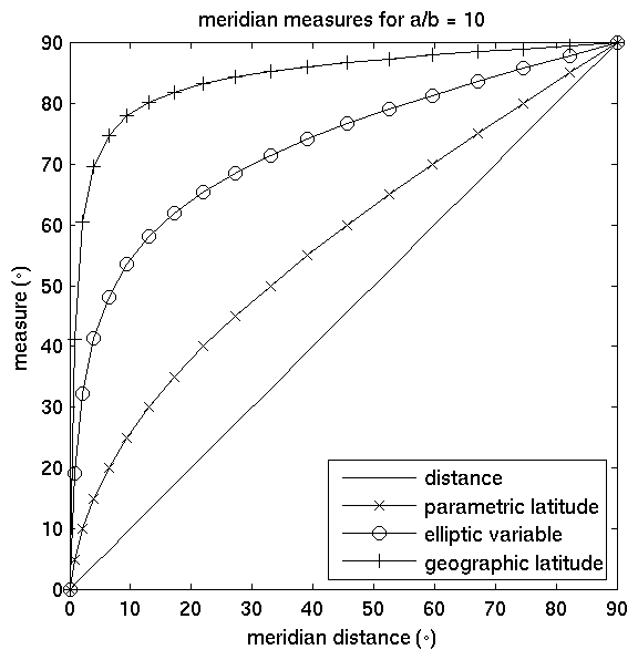
- For highly eccentric ellipsoids the variation of the meridian with respect to \( \beta \) is considerably "better behaved" than other choices (see the figure below). The choice of \( \phi \) is probably a poor one in this case.
GeographicLib uses the geodesic generalization of \( y = b E(\beta, ie') \), namely \( s = b E(\sigma, ik) \). See Geodesics in terms of elliptic integrals.
Short geodesics
Here we describe Bowring's method for solving the inverse geodesic problem in the limit of short geodesics and contrast it with the great circle solution using Bessel's auxiliary sphere. References:
- B. R. Bowring, The Direct and Inverse Problems for Short Geodesic Lines on the Ellipsoid, Surveying and Mapping 41(2), 135–141 (1981).
- R. H. Rapp, Geometric Geodesy, Part I, Ohio State Univ. (1991), Sec. 6.5.
Bowring considers the conformal mapping of the ellipsoid to a sphere of radius \( R \) such that circles of latitude and meridians are preserved (and hence the azimuth of a line is preserved). Let \( (\phi, \lambda) \) and \( (\phi', \lambda') \) be the latitude and longitude on the ellipsoid and sphere respectively. Define isometric latitudes for the sphere and the ellipsoid as
\[ \begin{align} \psi' &= \sinh^{-1} \tan \phi', \\ \psi &= \sinh^{-1} \tan \phi - e \tanh^{-1}(e \sin\phi). \end{align} \]
The most general conformal mapping satisfying Bowring's conditions is
\[ \psi' = A \psi + K, \quad \lambda' = A \lambda, \]
where \( A \) and \( K \) are constants. (In fact a constant can be added to the equation for \( \lambda' \), but this does affect the analysis.) The scale of this mapping is
\[ m(\phi) = \frac{AR}{\nu}\frac{\cos\phi'}{\cos\phi}, \]
where \( \nu = a/\sqrt{1 - e^2\sin^2\phi} \) is the transverse radius of curvature. (Note that in Bowring's Eq. (10), \( \phi \) should be replaced by \( \phi' \).) The mapping from the ellipsoid to the sphere depends on three parameters \( R, A, K \). These will be selected to satisfy certain conditions at some representative latitude \( \phi_0 \). Two possible choices are given below.
Bowring's method
Bowring (1981) requires that
\[ m(\phi_0) = 1,\quad \left.\frac{dm(\phi)}{d\phi}\right|_{\phi=\phi_0} = 0,\quad \left.\frac{d^2m(\phi)}{d\phi^2}\right|_{\phi=\phi_0} = 0, \]
i.e, \(m\approx 1\) in the vicinity of \(\phi = \phi_0\). This gives
\[ \begin{align} R &= \frac{\sqrt{1 + e'^2}}{B^2} a, \\ A &= \sqrt{1 + e'^2 \cos^4\phi_0}, \\ \tan\phi'_0 &= \frac1B \tan\phi_0, \end{align} \]
where \( e' = e/\sqrt{1-e^2} \) is the second eccentricity, \( B = \sqrt{1+e'^2\cos^2\phi_0} \), and \( K \) is defined implicitly by the equation for \(\phi'_0\). The radius \( R \) is the (Gaussian) mean radius of curvature of the ellipsoid at \(\phi_0\) (so near \(\phi_0\) the ellipsoid can be deformed to fit the sphere snugly). The third derivative of \( m \) is given by
\[ \left.\frac{d^3m(\phi)}{d\phi^3}\right|_{\phi=\phi_0} = \frac{-2e'^2\sin2\phi_0}{B^4}. \]
The method for solving the inverse problem between two nearby points \( (\phi_1, \lambda_1) \) and \( (\phi_2, \lambda_2) \) is as follows: Set \(\phi_0 = (\phi_1 + \phi_2)/2\). Compute \( R, A, \phi'_0 \), and hence find \( (\phi'_1, \lambda'_1) \) and \( (\phi'_2, \lambda'_2) \). Finally, solve for the great circle on a sphere of radius \( R \); the resulting distance and azimuths are good approximations for the corresponding quantities for the ellipsoidal geodesic.
Consistent with the accuracy of this method, we can compute \(\phi'_1\) and \(\phi'_2\) using a Taylor expansion about \(\phi_0\). This also avoids numerical errors that arise from subtracting nearly equal quantities when using the equation for \(\phi'\) directly. Write \(\Delta \phi = \phi - \phi_0\) and \(\Delta \phi' = \phi' - \phi'_0\); then we have
\[ \Delta\phi' \approx \frac{\Delta\phi}B \biggl[1 + \frac{\Delta\phi}{B^2}\frac{e'^2}2 \biggl(3\sin\phi_0\cos\phi_0 + \frac{\Delta\phi}{B^2} \bigl(B^2 - \sin^2\phi_0(2 - 3 e'^2 \cos^2\phi_0)\bigr)\biggr)\biggr], \]
where the error is \(O(f\Delta\phi^4)\). This is essentially Bowring's method. Significant differences between this result, "Bowring (improved)", compared to Bowring's paper, "Bowring (original)", are:
- Bowring elects to use \(\phi_0 = \phi_1\). This simplifies the calculations somewhat but increases the error by about a factor of 4.
- Bowring's expression for \( \Delta\phi' \) is only accurate in the limit \( e' \rightarrow 0 \).
In fact, arguably, the highest order \(O(f\Delta\phi^3)\) terms should be dropped altogether. Their inclusion does result in a better estimate for the distance. However, if your goal is to generate both accurate distances and accurate azimuths, then \(\Delta\phi\) needs to be restricted sufficiently to allow these terms to be dropped to give the "Bowring (truncated)" method.
With highly eccentric ellipsoids, the parametric latitude \( \beta \) is a better behaved independent variable to use. In this case, \( \phi_0 \) is naturally defined using \(\beta_0 = (\beta_1 + \beta_2)/2\) and in terms of \(\Delta\beta = \beta - \beta_0\), we have
\[ \Delta\phi' \approx \frac{\Delta\beta}{B'} \biggl[1 + \frac{\Delta\beta}{B'^2}\frac{e'^2}2 \biggl(\sin\beta_0\cos\beta_0 + \frac{\Delta\beta}{3B'^2} \bigl( \cos^2\beta_0 - \sin^2\beta_0 B'^2\bigr) \biggr)\biggr], \]
where \(B' = \sqrt{1+e'^2\sin^2\beta_0} = \sqrt{1+e'^2}/B\), and the error once again is \(O(f\Delta\phi^4)\). This is the "Bowring (using \(\beta\))" method.
Bessel's auxiliary sphere
GeographicLib's uses the auxiliary sphere method of Legendre, Bessel, and Helmert. For short geodesics, this is equivalent to picking \( R, A, K \) so that
\[ m(\phi_0) = 1,\quad \left.\frac{dm(\phi)}{d\phi}\right|_{\phi=\phi_0} = 0,\quad \tan\phi'_0 = (1 - f) \tan\phi_0. \]
Bowring's requirement that the second derivative of \(m\) vanish has been replaced by the last relation which states that \(\phi'_0 = \beta_0\), the parametric latitude corresponding to \(\phi_0\). This gives
\[ \begin{align} R &= B'(1-f)a, \\ A &= \frac1{B'(1-f)}, \\ \left.\frac{d^2m(\phi)}{d\phi^2}\right|_{\phi=\phi_0} &= -e^2B'^2\sin^2\phi_0. \end{align} \]
Similar to Bowring's method, we can compute \(\phi'_1\) and \(\phi'_2\) using a Taylor expansion about \(\beta_0\). This results in the simple expression
\[ \Delta\phi' \approx \Delta\beta, \]
where the error is \(O(f\Delta\beta^2)\).
Estimating the accuracy
In assessing the accuracy of these methods we use two metrics:
- The absolute error in the distance.
- The consistency of the predicted azimuths. Imagine starting ellipsoidal geodesics at \( (\phi_1, \lambda_1) \) and \( (\phi_2, \lambda_2) \) with the predicted azimuths. What is the distance between them when they are extended a distance \( a \) beyond the second point?
(The second metric is much more stringent.) We may now compare the methods by asking for a bound to the length of a geodesic which ensures that the one or other of the errors fall below 1 mm (an "engineering" definition of accurate) or 1 nm (1 nanometer, about the round-off limit).
| method | ||||
|---|---|---|---|---|
| 1 mm error | 1 nm error | 1 mm error | 1 nm error | |
| Bowring (original) | ||||
| Bowring (improved) | ||||
| Bowring (truncated) | ||||
| Bowring (using \(\beta\)) | ||||
| Bessel's aux. sphere | ||||
For example, if you're only interested in measuring distances and an accuracy of 1 mm is sufficient, then Bowring's improved method can be used for distances up to 180 km. On the other hand, GeographicLib uses Bessel's auxiliary sphere and we require both the distance and the azimuth to be accurate, so the great circle approximation can only be used for distances less than 1.7 m. The reason that GeographicLib does not use Bowring's method is that the information necessary for auxiliary sphere method is already available as part of the general solution and, as much as possible, we allow all geodesics to be computed by the general method.